Dynamic Programming Common Patterns and Code Template
This article will resolve
| LeetCode | Difficulty |
|---|---|
| 322. Coin Change | 🟠 |
| 509. Fibonacci Number | 🟢 |
Prerequisite Knowledge
Before reading this article, you should first learn:
Dynamic Programming (DP) problems can be challenging for many readers, but they are also among the most interesting and skillful types of problems. This site dedicates an entire chapter to this algorithm, which shows the importance of dynamic programming.
This article will address several questions:
- What is dynamic programming?
- What are the techniques to solve dynamic programming problems?
- How should you learn dynamic programming?
After solving many problems, you will notice that there are only a few main algorithm strategies. In the following chapters about dynamic programming, we will use the same problem-solving framework discussed here. If you understand the framework, tackling DP problems will become much easier. That is why this article is placed at the beginning, aiming to serve as a guide for solving dynamic programming problems. Now, let’s get to the main content.
First, the common form of a dynamic programming problem is to find an optimal value. Dynamic programming is actually an optimization technique from operations research, but it is widely used in computer science. For example, you may be asked to find the longest increasing subsequence, the minimum edit distance, and so on.
Since we are looking for an optimal value, what is the core issue? The core of solving a dynamic programming problem is enumeration (brute-force search). To find the optimal value, you have to enumerate all possible answers and then select the optimal one.
Is dynamic programming really that simple—just brute-force enumeration? But the DP problems I’ve seen are so difficult!
Although the main idea of dynamic programming is brute-force search for the optimal value, the problems can be very diverse. Enumerating all possible solutions is not easy; you need to be good at recursive thinking. Only by writing the correct "state transition equation" can you enumerate correctly.
In addition, you need to determine whether the problem has "optimal substructure", which means whether the optimal solution to the problem can be constructed from the optimal solutions to its subproblems.
Moreover, dynamic programming problems have "overlapping subproblems". If you use brute-force enumeration, the efficiency will be very low. Therefore, you need to use a "memoization" technique or a "DP table" to optimize the process and avoid unnecessary calculations.
The three key elements of dynamic programming are: overlapping subproblems, optimal substructure, and state transition equations. We will explain these in detail with examples. However, in practical algorithm problems, writing the state transition equation is usually the hardest part. Many people struggle with this, so I will share a thinking framework to help you develop state transition equations:
Clarify the "state" -> Clarify the "choices" -> Define the meaning of the dp array/function.
By following this framework, your final code will look like this:
# Top-down recursive dynamic programming
def dp(state1, state2, ...):
    for choice in all possible choices:
        # The state changes after making the choice
        result = find_optimal(result, dp(state1, state2, ...))
    return result

# Bottom-up iterative dynamic programming
# Initialize base case
dp[0][0][...] = base case
# Perform state transitions
for state1 in all possible values of state1:
    for state2 in all possible values of state2:
        for ...
            dp[state1][state2][...] = find_optimal(choice1, choice2, ...)
Next, we will use the Fibonacci problem and the coin change problem to explain the basic principles of dynamic programming. The first example will help you understand what overlapping subproblems are (although Fibonacci does not optimize for an optimal value, so strictly speaking, it is not a DP problem), and the second will focus on how to construct state transition equations.
1. Fibonacci Sequence
LeetCode Problem 509 "Fibonacci Number" is about this problem. Please don't be discouraged by the simplicity of this example. Only simple examples allow you to focus fully on the underlying ideas and techniques of the algorithm, without getting distracted by tricky details. If you want more challenging examples, there will be plenty in the upcoming dynamic programming series.
Brute-force Recursion
The mathematical definition of the Fibonacci sequence is recursive. The code implementation is as follows:
// f(n) calculates the nth Fibonacci number
int fib(int n) {
    // base case
    if (n == 0 || n == 1){
        return n;
    }
    return fib(n - 1) + fib(n - 2);
}// f(n) calculates the nth Fibonacci number
int fib(int n) {
// base case
if (n == 0 || n == 1){
return n;
}
return fib(n - 1) + fib(n - 2);
}# f(n) calculates the nth Fibonacci number
def fib(n: int) -> int:
# base case
if n == 0 or n == 1:
return n
return fib(n - 1) + fib(n - 2)// f(n) calculates the nth Fibonacci number
func fib(n int) int {
// base case
if n == 0 || n == 1 {
return n
}
return fib(n-1) + fib(n-2)
}// f(n) calculates the nth Fibonacci number
var fib = function(n) {
// base case
if (n == 0 || n == 1) {
return n;
}
return fib(n - 1) + fib(n - 2);
};Info
According to the LeetCode problem description, the base cases are f(0) = 0 and f(1) = 1. In some other definitions, the base cases are f(1) = 1 and f(2) = 1. In fact, these are equivalent.
When teaching recursion, school teachers often use this as an example. We also know that although this code is simple and easy to understand, it is very inefficient. Why is it inefficient? Suppose n = 20. Let's draw the recursion tree:
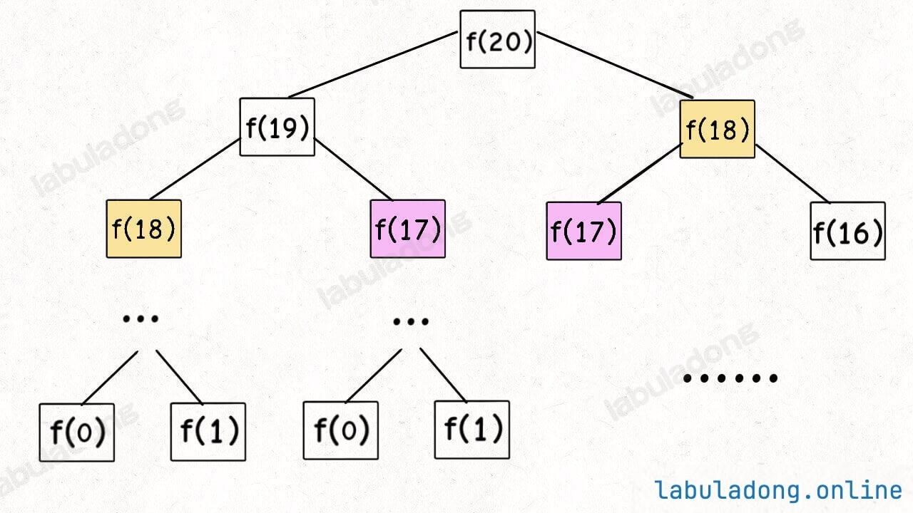
How do we understand this recursion tree? To compute the original problem f(20), we first need to compute the subproblems f(19) and f(18). To compute f(19), we need to compute f(18) and f(17), and so on. When we reach f(1) or f(2), we already know the results, so we can return immediately, and the recursion tree does not grow further downward.
Using an algorithm visualization tool can help you understand this process better. The recursion tree for f(20) is too large, so let's look at the recursion process for f(5).
Please open the visualization panel below and click the line if (n == 0 || n == 1). You will see the recursion tree grow downward, and when it reaches a leaf node (base case), it returns the result layer by layer:
Algorithm Visualization
How do we calculate the time complexity of a recursive algorithm? Multiply the number of subproblems by the time needed to solve each subproblem.
First, count the number of subproblems, which is the total number of nodes in the recursion tree. The height of this recursion tree is , so the total number of nodes in a binary tree is .
Next, calculate the time needed to solve a subproblem. In this algorithm, there are no loops, only one addition operation f(n - 1) + f(n - 2), which takes time.
Therefore, the total time complexity is the product of the two, which is —exponential time, which can quickly become unmanageable.
Looking at the recursion tree, it is clear why the algorithm is inefficient: there is a lot of repeated computation.
For example, f(18) is calculated twice, and as you can see, the subtree rooted at f(18) is quite large. Recomputing it wastes a lot of time. And f(18) is not the only node that gets recalculated, so the algorithm is very inefficient.
This demonstrates the first property of dynamic programming problems: overlapping subproblems. Next, we will look for ways to solve this issue.
Recursive Solution with Memoization
Since the main cause of inefficiency is repeated calculations, we can create a "memoization" table. Each time we solve a subproblem, we save the answer in the memoization table. When we encounter a subproblem, we first check the table. If the answer has already been computed, we simply return it instead of recalculating.
For the Fibonacci problem, we need a memoization table to record the value of the subproblem f(x), where x is a non-negative integer. We usually use a one-dimensional array memo as the memoization table, where memo[x] stores the answer for subproblem f(x).
Of course, you can also use a hash table for storage. The idea is the same.
int fib(int n) {
    // initialize the memo array to all -1
    // because the Fibonacci number is a non-negative integer, so
    // initialize it with -1 to indicate that it has not been calculated

    // because the index of the array starts at 0, so we need n + 1 spaces
    // so we can record `f(0) ~ f(n)` in memo
    int[] memo = new int[n + 1];
    Arrays.fill(memo, -1);

    return dp(memo, n);
}

// perform recursion with memoization
int dp(int[] memo, int n) {
    // base case
    if (n == 0 || n == 1) {
        return n;
    }
    // already calculated, no need to calculate again
    if (memo[n] != -1) {
        return memo[n];
    }
    // before returning the result, store it in the memo
    memo[n] = dp(memo, n - 1) + dp(memo, n - 2);
    return memo[n];
}int fib(int n) {
// initialize the memo array to all -1
// because the Fibonacci number is a non-negative integer, so
// initialize it with -1 to indicate that it has not been calculated
// because the index of the array starts at 0, so we need n + 1 spaces
// so we can record `f(0) ~ f(n)` in memo
vector<int> memo(n + 1, -1);
// perform recursion with memoization
return dp(memo, n);
}
// perform recursion with memoization
int dp(vector<int>& memo, int n) {
// base case
if (n == 0 || n == 1) {
return n;
}
// already calculated, no need to calculate again
if (memo[n] != -1) {
return memo[n];
}
// before returning the result, store it in the memo
memo[n] = dp(memo, n - 1) + dp(memo, n - 2);
return memo[n];
}def fib(n: int) -> int:
# initialize the memo array to all -1
# because the Fibonacci number is a non-negative integer, so
# initialize it with -1 to indicate that it has not been calculated
# because the index of the array starts at 0, so we need n + 1 spaces
# so we can record `f(0) ~ f(n)` in memo
memo = [-1] * (n + 1)
return self.dp(memo, n)
# perform recursion with memoization
def dp(memo: list, n: int) -> int:
# base case
if n == 0 or n == 1:
return n
# already calculated, no need to calculate again
if memo[n] != -1:
return memo[n]
# before returning the result, store it in the memo
memo[n] = self.dp(memo, n - 1) + self.dp(memo, n - 2)
return memo[n]func fib(n int) int {
// initialize the memo array to all -1
// because the Fibonacci number is a non-negative integer, so
// initialize it with -1 to indicate that it has not been calculated
// because the index of the array starts at 0, so we need n + 1 spaces
// so we can record `f(0) ~ f(n)` in memo
memo := make([]int, n+1)
for i := range memo {
memo[i] = -1
}
return dp(memo, n)
}
// perform recursion with memoization
func dp(memo []int, n int) int {
// base case
if n == 0 || n == 1 {
return n
}
// already calculated, no need to calculate again
if memo[n] != -1 {
return memo[n]
}
// before returning the result, store it in the memo
memo[n] = dp(memo, n-1) + dp(memo, n-2)
return memo[n]
}var fib = function(n) {
// initialize the memo array to all -1
// because the Fibonacci number is a non-negative integer, so
// initialize it with -1 to indicate that it has not been calculated
// because the index of the array starts at 0, so we need n + 1 spaces
// so we can record `f(0) ~ f(n)` in memo
let memo = new Array(n + 1).fill(-1);
return dp(memo, n);
};
// perform recursion with memoization
var dp = function(memo, n) {
// base case
if (n === 0 || n === 1) {
return n;
}
// already calculated, no need to calculate again
if (memo[n] !== -1) {
return memo[n];
}
// before returning the result, store it in the memo
memo[n] = dp(memo, n - 1) + dp(memo, n - 2);
return memo[n];
}Now, let's draw the recursion tree to see what memoization actually does.
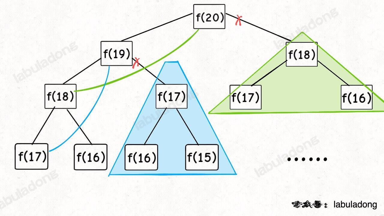
In fact, recursive algorithms with memoization prune away the redundant branches of the recursion tree, turning it into a recursion graph without redundancy. This greatly reduces the number of subproblems (nodes in the graph), and each subproblem is calculated only once:
How do you calculate the time complexity of a recursive algorithm? Multiply the number of subproblems by the time needed to solve each subproblem.
The number of subproblems is the total number of nodes in the graph. Since this algorithm avoids redundant calculations, the subproblems are simply f(0), f(1), f(2), ..., f(20). The number of subproblems is proportional to the input size n = 20, so there are subproblems.
The time to solve each subproblem is , as there are no loops inside.
Therefore, the overall time complexity of this algorithm is , which is much more efficient than the exponential time complexity of brute-force solutions.
Here, you can also use the algorithm visualization panel to see the effect of pruning. The recursion tree of fib(20) is too large, so let's look at the recursion process of fib(5).
Please open this visualization panel and click the line if (n == 0 || n == 1) multiple times to observe the growth of the recursion tree. Notice that when encountering duplicate nodes, the recursion tree stops growing downward and directly returns the result. This is the effect of pruning.
Algorithm Visualization
Top-Down vs Bottom-Up
If you have mastered the content above, you already know how to solve dynamic programming problems: start with a brute-force solution, then use a "memoization" technique to prune and eliminate overlapping subproblems. Dynamic programming is just that simple.
However, some readers may ask: why do many dynamic programming solutions I see only use several for loops, without any recursion or memoization? What is going on here?
In fact, there are two main approaches to dynamic programming:
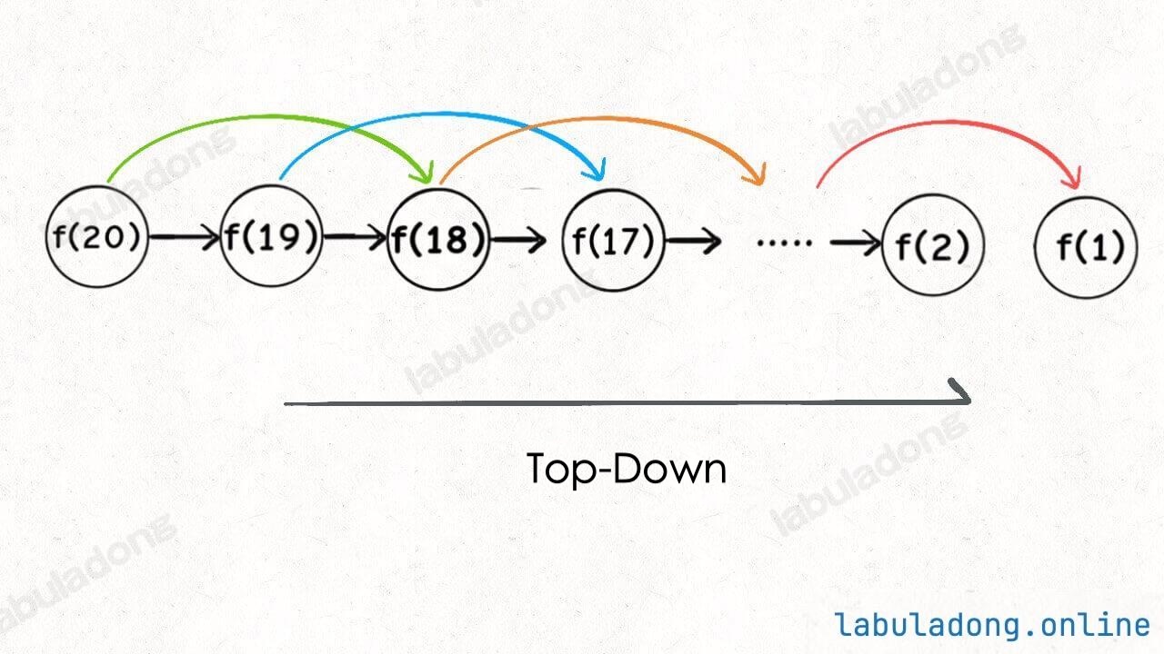
The first is the recursive solution with memoization, also known as the "top-down" approach, which we showed above—a recursive function with a memo array.
The second is the iterative solution with a DP table, also called the "bottom-up" approach. This is what you described: using for loops to fill out a dp array.
These two approaches are essentially the same and can be converted into each other. The dp array in the iterative solution is the same as the memo array in the recursive solution.
Why is it called "top-down"? For example, in the recursive solution above, if you click if (n == 0 || n == 1) multiple times, you can see the recursion tree growing from top to bottom. It starts from the original problem f(5) and breaks it down into smaller problems until it reaches the base cases f(0) and f(1), then returns the answers layer by layer. This is called "top-down".
Algorithm Visualization
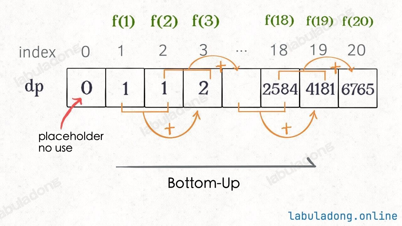
What is "bottom-up"? It is the opposite. We start from the simplest, smallest subproblems with known results—f(0) and f(1) (the base cases)—and work our way up to find f(2), f(3), ..., until we reach f(5). This is "bottom-up".
In fact, "top-down" and "bottom-up" are essentially the same, just from different perspectives.
For example, if we slightly modify the recursive solution with memoization above, and move the base case handling (n == 0 || n == 1) from the recursive function dp into the memo array, it should be fine. Let's look again at the calculation process of fib(5).
You can click on memo[n] = dp(memo, n - 1) + dp(memo, n - 2) multiple times. Pay attention to the changes in the recursion tree and the memo array:
Algorithm Visualization
You can see that the process of passing results up the recursion tree is just the same as calculating the memo array from the base cases to the right. This is the bottom-up approach, and it is very intuitive.
By now, you might have noticed that the entire computation is just calculating the values in memo from left to right. Why bother using recursion, making things more complex? Isn't a for loop enough?
Iterative DP Array Solution
With this insight, we no longer need to use recursion. We simply create an array (the DP table) and use a for loop to calculate values from the base cases from left to right.
int fib(int n) {
    if (n == 0 || n == 1) {
        return n;
    }
    // dp table
    int[] dp = new int[n + 1];
    // base case
    dp[0] = 0; dp[1] = 1;
    // state transition
    for (int i = 2; i <= n; i++) {
        dp[i] = dp[i - 1] + dp[i - 2];
    }

    return dp[n];
}int fib(int n) {
if (n == 0 || n == 1) {
return n;
}
// dp table
vector<int> dp(n + 1);
// base case
dp[0] = 0; dp[1] = 1;
// state transition
for (int i = 2; i <= n; i++) {
dp[i] = dp[i - 1] + dp[i - 2];
}
return dp[n];
}def fib(n: int) -> int:
if n == 0 or n == 1:
return n
# dp table
dp = [0] * (n + 1)
# base case
dp[0] = 0
dp[1] = 1
# state transition
for i in range(2, n + 1):
dp[i] = dp[i - 1] + dp[i - 2]
return dp[n]func fib(n int) int {
if n == 0 || n == 1 {
return n
}
// dp table
dp := make([]int, n+1)
// base case
dp[0], dp[1] = 0, 1
// state transition
for i := 2; i <= n; i++ {
dp[i] = dp[i-1] + dp[i-2]
}
return dp[n]
}var fib = function(n) {
if (n === 0 || n === 1) {
return n;
}
// dp table
let dp = new Array(n + 1).fill(0);
// base case
dp[0] = 0; dp[1] = 1;
// state transition
for (let i = 2; i <= n; i++) {
dp[i] = dp[i - 1] + dp[i - 2];
}
return dp[n];
};Algorithm Visualization
The diagram makes this approach easy to understand, and you can see that this DP table is similar to the "pruned" result from before, just calculated in the opposite direction:
In fact, the "memo" array in the recursive solution with memoization ends up being the same as the dp array in this solution. If you compare the visualizations of the two algorithms, you can clearly see their connection.
So, the top-down and bottom-up approaches are essentially the same, and in most cases, their efficiency is about the same.
Further Exploration
Here, let's introduce the concept of the "state transition equation," which is simply the mathematical way to describe the structure of a problem:
Why is it called a "state transition equation"? The name just sounds fancy.
The function parameter f(n) keeps changing, so you can think of the parameter n as a "state." This state n is derived (by addition) from states n - 1 and n - 2. This process is called a state transition, and that's all there is to it.
You will notice that all the operations in the solutions above, such as return f(n - 1) + f(n - 2), dp[i] = dp[i - 1] + dp[i - 2], and the initialization of a memoization array or DP table, are different forms of this same equation.
This shows how important it is to write out the "state transition equation." It is the core of solving the problem, and it is easy to see that the equation itself represents the brute-force solution.
Never look down on the brute-force solution. The hardest part of dynamic programming is writing out this brute-force solution, which is the state transition equation.
Once you have the brute-force solution, the only way to optimize it is to use memoization or a DP table. There are no more mysteries after that.
Now, let's discuss a detail for optimization.
Careful readers may notice that according to the state transition equation for the Fibonacci sequence, the current state n only depends on the previous two states, n-1 and n-2. Therefore, you do not need a long DP table to store all the states. You just need to find a way to store the previous two states.
So, you can further optimize and reduce the space complexity to . This is the most common algorithm for computing Fibonacci numbers:
int fib(int n) {
    if (n == 0 || n == 1) {
        // base case
        return n;
    }
    // represent dp[i - 1] and dp[i - 2] respectively
    int dp_i_1 = 1, dp_i_2 = 0;
    for (int i = 2; i <= n; i++) {
        // dp[i] = dp[i - 1] + dp[i - 2];
        int dp_i = dp_i_1 + dp_i_2;
        // rolling update
        dp_i_2 = dp_i_1;
        dp_i_1 = dp_i;
    }
    return dp_i_1;
}int fib(int n) {
if (n == 0 || n == 1) {
// base case
return n;
}
// represent dp[i - 1] and dp[i - 2] respectively
int dp_i_1 = 1, dp_i_2 = 0;
for (int i = 2; i <= n; i++) {
// dp[i] = dp[i - 1] + dp[i - 2];
int dp_i = dp_i_1 + dp_i_2;
// rolling update
dp_i_2 = dp_i_1;
dp_i_1 = dp_i;
}
return dp_i_1;
}def fib(n: int) -> int:
if n == 0 or n == 1:
# base case
return n
# represent dp[i - 1] and dp[i - 2] respectively
dp_i_1, dp_i_2 = 1, 0
for i in range(2, n + 1):
# dp[i] = dp[i - 1] + dp[i - 2];
dp_i = dp_i_1 + dp_i_2
# rolling update
dp_i_2 = dp_i_1
dp_i_1 = dp_i
return dp_i_1func fib(n int) int {
if n == 0 || n == 1 {
// base case
return n
}
// represent dp[i - 1] and dp[i - 2] respectively
dp_i_1, dp_i_2 := 1, 0
for i := 2; i <= n; i++ {
// dp[i] = dp[i - 1] + dp[i - 2];
dp_i := dp_i_1 + dp_i_2
// rolling update
dp_i_2 = dp_i_1
dp_i_1 = dp_i
}
return dp_i_1
}var fib = function(n) {
if (n === 0 || n === 1) {
// base case
return n;
}
// represent dp[i - 1] and dp[i - 2] respectively
let dp_i_1 = 1, dp_i_2 = 0;
for (let i = 2; i <= n; i++) {
// dp[i] = dp[i - 1] + dp[i - 2];
let dp_i = dp_i_1 + dp_i_2;
// rolling update
dp_i_2 = dp_i_1;
dp_i_1 = dp_i;
}
return dp_i_1;
};Algorithm Visualization
This is usually the final step of optimization for dynamic programming problems. If you find that each state transition only needs part of the DP table, you can try to shrink the size of the DP table and record only the necessary data, thereby lowering the space complexity.
In the example above, the size of the DP table is reduced from n to 2, which reduces the space complexity by an order of magnitude. I will explain more about this technique for reducing space complexity in the article Reducing the Dimension of Dynamic Programming. Generally, it is used to compress a two-dimensional DP table into one dimension, reducing the space complexity from to .
Some might ask: What about another important property of dynamic programming, the "optimal substructure"? Why isn't it discussed here? It will be covered below. Strictly speaking, the Fibonacci sequence is not a real dynamic programming problem because it does not involve finding an optimal value. The example above is mainly to show how to eliminate overlapping subproblems and demonstrate the process of step-by-step refinement of the optimal solution. Next, let's look at the second example: the coin change problem.
2. Coin Change Problem
This is LeetCode Problem 322: Coin Change:
You are given k types of coins, with denominations c1, c2 ... ck. Each type of coin has an unlimited supply. Given a total amount amount, find the minimum number of coins needed to make up that amount. If it is not possible, return -1. The function signature is as follows:
// `coins` contains the denominations of available coins, and `amount` is the target amount
int coinChange(int[] coins, int amount);// coins contains the denominations of available coins, and amount is the target amount
int coinChange(vector<int>& coins, int amount);# coins contains the denominations of available coins, amount is the target amount
def coinChange(coins: List[int], amount: int) -> int:// coins contains the denominations of available coins, and amount is the target amount
func coinChange(coins []int, amount int) int {}var coinChange = function(coins, amount) {}For example, if k = 3, the denominations are 1, 2, and 5, and the total amount amount = 11. The minimum number of coins required is 3, that is, 11 = 5 + 5 + 1.
How should a computer solve this problem? Clearly, we can enumerate all possible combinations of coins and find the one that uses the fewest coins.
Brute-force Recursion
First, this is a dynamic programming problem because it has an "optimal substructure." For the optimal substructure to hold, the subproblems must be independent of each other. What does it mean to be independent? Instead of a mathematical proof, let's look at an intuitive example.
Suppose you are taking an exam, and the scores of each subject are independent. Your main goal is to achieve the highest total score. Your subproblems are to get the highest score in Chinese, the highest in Math, and so on. To get the highest score in each subject, you need to get the highest possible score in each section, like multiple choice and fill-in-the-blank. In the end, if you score full marks in every subject, you achieve the highest total score.
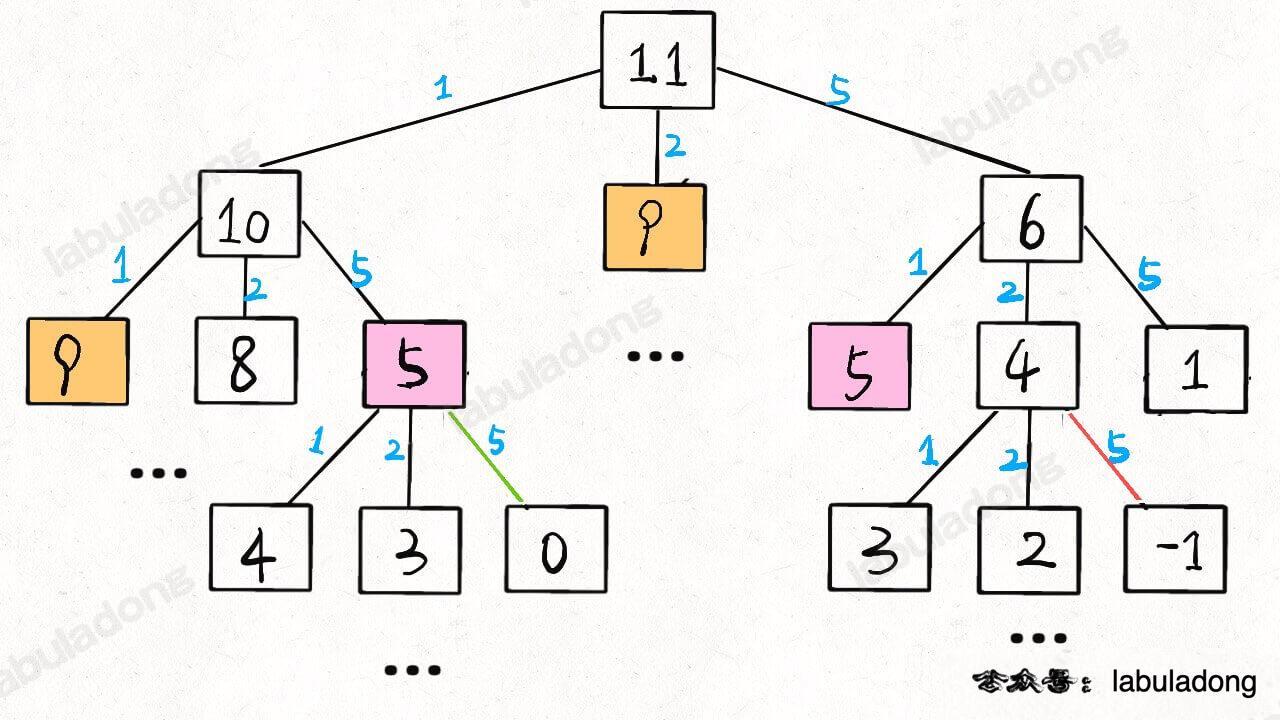
This gives the correct result: the highest total score is the sum of the highest scores in each subject. This works because the subproblems are independent and do not interfere with each other, so the problem has an optimal substructure.
However, if there is a new condition: your Chinese and Math scores affect each other and cannot both be full marks; if your Math score is high, your Chinese score goes down, and vice versa.
In this case, clearly, you cannot achieve the full total score, and the previous approach will give the wrong result. This is because the subproblems are not independent—Chinese and Math scores affect each other, so the optimal substructure is broken.
Back to the coin change problem, why does it have an optimal substructure? Suppose you have coins with denominations 1, 2, 5, and you want to find the minimum number of coins needed for amount = 11 (the main problem). If you already know the minimum number of coins needed for amount = 10, 9, 6 (the subproblems), you just add one more coin (of value 1, 2, or 5) to those subproblems and take the minimum result. Because you have an unlimited supply of each coin, the subproblems are independent of each other.
Tip
For more examples about the optimal substructure property, see Dynamic Programming Q&A later in this article.
Now that we know this is a dynamic programming problem, how do we write the correct state transition equation?
1. Determine the "state", which refers to the variables that change in the original problem and its subproblems. Since the number of coins is unlimited and the coin denominations are provided by the problem, only the target amount keeps moving closer to the base case. So the only "state" is the target amount amount.
2. Determine the "choices", which are the actions that cause the "state" to change. Why does the target amount change? Because you are choosing coins. Each time you pick a coin, you reduce the target amount by the value of that coin. Therefore, the denominations of all coins are your "choices".
3. Define the dp function/array. Here we are using the top-down approach, so we will have a recursive dp function. Usually, the parameters of the function are the variables that change during the state transition, i.e., the "state" mentioned above. The return value of the function is the quantity the problem requires us to compute. For this problem, the only state is the "target amount", and the problem requires us to calculate the minimum number of coins needed to make up the target amount.
So, we can define the dp function like this: dp(n) means, given a target amount n, return the fewest number of coins needed to make up amount n.
According to this definition, our final answer is the return value of dp(amount).
Once you understand these key points, you can write the pseudocode for the solution:
// Pseudocode framework
int coinChange(int[] coins, int amount) {
    // The final result required by the problem is dp(amount)
    return dp(coins, amount);
}

// Definition: To make up the amount n, at least dp(coins, n) coins are needed
int dp(int[] coins, int n) {
    // Make a choice, choose the result that requires the fewest coins
    for (int coin : coins) {
        res = min(res, 1 + dp(coins, n - coin));
    }
    return res;
}// Pseudocode framework
int coinChange(vector<int>& coins, int amount) {
// The final result required by the problem is dp(amount)
return dp(coins, amount);
}
// Definition: To make up the amount n, at least dp(coins, n) coins are needed
int dp(vector<int>& coins, int n) {
// Make a choice, choose the result that requires the fewest coins
int res = INT_MAX;
for (const int coin : coins) {
res = min(res, subProb + 1);
}
return res;
}# Pseudocode framework
def coinChange(coins: List[int], amount: int) -> int:
# The final result required by the problem is dp(amount)
return dp(coins, amount)
# Definition: To make up the amount n, at least dp(coins, n) coins are needed
def dp(coins: List[int], n: int) -> int:
# Make a choice, choose the result that requires the fewest coins
# Initialize res to positive infinity
res = float('inf')
for coin in coins:
res = min(res, sub_problem + 1)
return res// Pseudocode framework
func coinChange(coins []int, amount int) int {
// The final result required by the problem is dp(amount)
return dp(coins, amount)
}
// Definition: To make up the amount n, at least dp(coins, n) coins are needed
func dp(coins []int, n int) int {
// Initialize to the maximum value
res := math.MaxInt32
// Make a choice, choose the result that requires the fewest coins
for _, coin := range coins {
res = min(res, 1+subProblem)
}
return res
}// Pseudocode framework
var coinChange = function(coins, amount) {
// The final result required by the problem is dp(amount)
return dp(coins, amount);
}
// Definition: To make up the amount n, at least dp(coins, n) coins are needed
var dp = function(coins, n) {
// Initialize to the maximum value
let res = Infinity;
// Make a choice, choose the result that requires the fewest coins
for (let coin of coins) {
res = Math.min(res, 1 + subProblem);
}
return res;
};Based on the pseudocode, we add the base cases to get the final solution. Obviously, when the target amount is 0, the minimum number of coins needed is 0. When the target amount is less than 0, there is no solution, so return -1:
class Solution {
    public int coinChange(int[] coins, int amount) {
        // the final result required by the problem is dp(amount)
        return dp(coins, amount);
    }

    // definition: to make up the `amount`, at least dp(coins, amount) coins are needed
    int dp(int[] coins, int amount) {
        // base case
        if (amount == 0) return 0;
        if (amount < 0) return -1;

        int res = Integer.MAX_VALUE;
        for (int coin : coins) {
            // calculate the result of the subproblem
            int subProblem = dp(coins, amount - coin);
            // skip if the subproblem has no solution
            if (subProblem == -1) continue;
            // choose the optimal solution from the subproblem, then add one
            res = Math.min(res, subProblem + 1);
        }

        return res == Integer.MAX_VALUE ? -1 : res;
    }
}class Solution {
public:
int coinChange(vector<int>& coins, int amount) {
// the final result required by the problem is dp(amount)
return dp(coins, amount);
}
private:
// definition: to make up the `amount`, at least dp(coins, amount) coins are needed
int dp(vector<int>& coins, int amount) {
// base case
if (amount == 0) return 0;
if (amount < 0) return -1;
int res = INT_MAX;
for (int coin : coins) {
// calculate the result of the subproblem
int subProblem = dp(coins, amount - coin);
// skip if the subproblem has no solution
if (subProblem == -1) continue;
// choose the optimal solution in the subproblem, then add one
res = min(res, subProblem + 1);
}
return res == INT_MAX ? -1 : res;
}
};class Solution:
def coinChange(self, coins: List[int], amount: int) -> int:
# the final result required by the problem is dp(amount)
return self.dp(coins, amount)
# definition: to make up the `amount`, at least dp(coins, amount) coins are needed
def dp(self, coins, amount):
# base case
if amount == 0:
return 0
if amount < 0:
return -1
res = float('inf')
for coin in coins:
# calculate the result of the subproblem
subProblem = self.dp(coins, amount - coin)
# skip if the subproblem has no solution
if subProblem == -1:
continue
# choose the optimal solution in the subproblem, then add one
res = min(res, subProblem + 1)
return res if res != float('inf') else -1func coinChange(coins []int, amount int) int {
// The final result required by the problem is dp(amount)
return dp(coins, amount)
}
// Definition: to make up the `amount`, at least dp(coins, amount) coins are needed
func dp(coins []int, amount int) int {
// base case
if amount == 0 {
return 0
}
if amount < 0 {
return -1
}
res := math.MaxInt32
for _, coin := range coins {
// Calculate the result of the subproblem
subProblem := dp(coins, amount - coin)
// Skip if the subproblem has no solution
if subProblem == -1 {
continue
}
// Choose the optimal solution in the subproblem, then add one
res = min(res, subProblem + 1)
}
if res == math.MaxInt32 {
return -1
}
return res
}
func min(x, y int) int {
if x < y {
return x
}
return y
}var coinChange = function(coins, amount) {
// The final result required by the problem is dp(amount)
return dp(coins, amount);
}
// Definition: to make up the `amount`, at least dp(coins, amount) coins are needed
function dp(coins, amount) {
// base case
if (amount === 0) return 0;
if (amount < 0) return -1;
let res = Number.MAX_SAFE_INTEGER;
for (let coin of coins) {
// Calculate the result of the subproblem
let subProblem = dp(coins, amount - coin);
// Skip if the subproblem has no solution
if (subProblem === -1) continue;
// Choose the optimal solution in the subproblem, then add one
res = Math.min(res, subProblem + 1);
}
return res === Number.MAX_SAFE_INTEGER ? -1 : res;
}Info
Here, the signature of coinChange and the dp function are exactly the same, so in theory you don't need to write a separate dp function. However, for clarity in later explanations, we still implement the main logic in a separate dp function.
Additionally, I often see readers ask: why do we add 1 to the result of the subproblem (subProblem + 1), instead of adding the coin's denomination or something else? Here is a general reminder: the key to dynamic programming problems is the definition of the dp function/array. What does your function's return value represent? Go back and make sure you understand this, and you will know why we add 1 to the result of the subproblem.
Algorithm Visualization
At this point, the state transition equation is actually complete. The above algorithm is a brute-force solution, and its mathematical form is the state transition equation:
So, the problem is basically solved. The only thing left is to eliminate overlapping subproblems. For example, when amount = 11 and coins = {1,2,5}, you can draw out the recursion tree to see:
Time complexity analysis of the recursive algorithm: total number of subproblems × time required to solve each subproblem.
The total number of subproblems is the number of nodes in the recursion tree. The algorithm will perform pruning, and the timing of pruning depends on the specific coin denominations given in the problem. So, you can imagine that the tree does not grow regularly, and it is difficult to compute the exact number of nodes. In this case, we usually estimate the upper bound of the time complexity in the worst case.
Assume the target amount is n, and there are k types of coins. In the worst case, the height of the recursion tree is n (all coins are of denomination 1). Assuming this is a full k-ary tree, the total number of nodes is on the order of k^n.
Next, consider the complexity for each subproblem. Since each recursion contains a for loop, the complexity is . Multiply them to get a total time complexity of , which is exponential.
Recursive Solution with Memoization
Similar to the previous Fibonacci example, with slight modification, we can use memoization to eliminate redundant subproblems:
class Solution {
    int[] memo;

    public int coinChange(int[] coins, int amount) {
        memo = new int[amount + 1];
        // Initialize the memo with a special value that won't be
        // picked, representing it has not been calculated
        Arrays.fill(memo, -666);

        return dp(coins, amount);
    }

    int dp(int[] coins, int amount) {
        if (amount == 0) return 0;
        if (amount < 0) return -1;
        // Check the memo to prevent repeated calculations
        if (memo[amount] != -666)
            return memo[amount];

        int res = Integer.MAX_VALUE;
        for (int coin : coins) {
            // Calculate the result of the subproblem
            int subProblem = dp(coins, amount - coin);
            // Skip if the subproblem has no solution
            if (subProblem == -1) continue;
            // Choose the optimal solution in the subproblem, then add one
            res = Math.min(res, subProblem + 1);
        }
        // Store the calculation result in the memo
        memo[amount] = (res == Integer.MAX_VALUE) ? -1 : res;
        return memo[amount];
    }
}class Solution {
public:
vector<int> memo;
int coinChange(vector<int>& coins, int amount) {
memo = vector<int> (amount + 1, -666);
// Initialize the memo with a special value that won't be
// picked, representing it has not been calculated
return dp(coins, amount);
}
int dp(vector<int>& coins, int amount) {
if (amount == 0) return 0;
if (amount < 0) return -1;
// Check the memo to prevent repeated calculations
if (memo[amount] != -666)
return memo[amount];
int res = INT_MAX;
for (int coin : coins) {
// Calculate the result of the subproblem
int subProblem = dp(coins, amount - coin);
// Skip if the subproblem has no solution
if (subProblem == -1) continue;
// Choose the optimal solution from the subproblems and add one
res = min(res, subProblem + 1);
}
// Store the calculation result in the memo
memo[amount] = (res == INT_MAX) ? -1 : res;
return memo[amount];
}
};class Solution:
def __init__(self):
self.memo = []
def coinChange(self, coins: List[int], amount: int) -> int:
self.memo = [-666] * (amount + 1)
# Initialize the memo with a special value that won't be
# picked, representing it has not been calculated
return self.dp(coins, amount)
def dp(self, coins, amount):
if amount == 0: return 0
if amount < 0: return -1
# Check the memo to prevent repeated calculations
if self.memo[amount] != -666:
return self.memo[amount]
res = float('inf')
for coin in coins:
# Calculate the result of the subproblem
subProblem = self.dp(coins, amount - coin)
# Skip if the subproblem has no solution
if subProblem == -1: continue
# Choose the optimal solution from the subproblems and add one
res = min(res, subProblem + 1)
# Store the calculation result in the memo
self.memo[amount] = res if res != float('inf') else -1
return self.memo[amount]import "math"
func coinChange(coins []int, amount int) int {
memo := make([]int, amount + 1)
for i := range memo {
memo[i] = -666
}
// Initialize the memo with a special value that won't be
// taken, representing that it has not been calculated
return dp(coins, amount, memo)
}
func dp(coins []int, amount int, memo []int) int {
if amount == 0 {
return 0
}
if amount < 0 {
return -1
}
// Check the memo to prevent repeated calculations
if memo[amount] != -666 {
return memo[amount]
}
res := math.MaxInt32
for _, coin := range coins {
// Calculate the result of the subproblem
subProblem := dp(coins, amount - coin, memo)
// Skip if the subproblem has no solution
if subProblem == -1 {
continue
}
// Choose the optimal solution in the subproblem and then add one
res = min(res, subProblem + 1)
}
// Store the calculation result in the memo
if res == math.MaxInt32 {
memo[amount] = -1
} else {
memo[amount] = res
}
return memo[amount]
}var coinChange = function(coins, amount) {
let memo = new Array(amount + 1).fill(-666);
// Initialize the memo with a special value that won't be
// picked, representing it has not been calculated
return dp(coins, amount, memo);
}
function dp(coins, amount, memo) {
if (amount === 0) return 0;
if (amount < 0) return -1;
// Check the memo to prevent repeated calculations
if (memo[amount] !== -666) {
return memo[amount];
}
let res = Infinity;
for (let coin of coins) {
// Calculate the result of the subproblem
let subProblem = dp(coins, amount - coin, memo);
// Skip if the subproblem has no solution
if (subProblem === -1) continue;
// Choose the optimal solution from the subproblem and add one
res = Math.min(res, subProblem + 1);
}
// Store the calculation result in the memo
memo[amount] = res === Infinity ? -1 : res;
return memo[amount];
}Algorithm Visualization
Without showing the diagram, it is clear that memoization greatly reduces the number of subproblems and completely removes redundancy. Therefore, the total number of subproblems will not exceed the amount n, making the number of subproblems . The time to process each subproblem remains , so the total time complexity is .
Iterative Solution Using dp Array
Of course, we can also use a bottom-up approach with a dp table to eliminate overlapping subproblems. The concepts of "state", "choice", and base case remain the same as before. The definition of the dp array is similar to the previous dp function; both use the target amount as a variable. The dp function uses function arguments, while the dp array uses array indices:
Definition of the dp array: When the target amount is i, dp[i] represents the minimum number of coins needed to make up the amount.
Based on the dynamic programming framework provided at the beginning of this article, we can write the following solution:
class Solution {
public int coinChange(int[] coins, int amount) {
int[] dp = new int[amount + 1];
// The array size is amount + 1, and the initial value is also amount + 1
Arrays.fill(dp, amount + 1);
// base case
dp[0] = 0;
// The outer for loop traverses all possible values of all states
for (int i = 0; i < dp.length; i++) {
// The inner for loop finds the minimum value among all choices
for (int coin : coins) {
// The subproblem has no solution, skip
if (i - coin < 0) {
continue;
}
dp[i] = Math.min(dp[i], 1 + dp[i - coin]);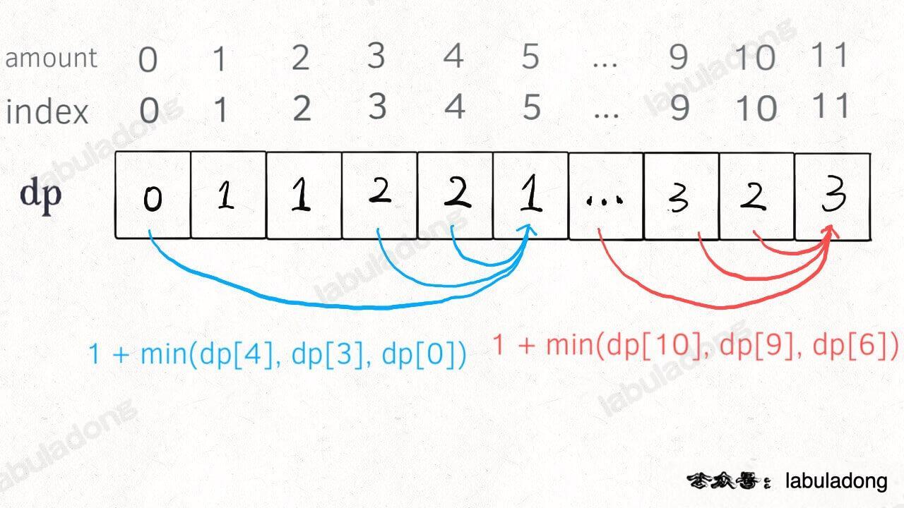 }
}
return (dp[amount] == amount + 1) ? -1 : dp[amount];
}
}
}
}
return (dp[amount] == amount + 1) ? -1 : dp[amount];
}
}class Solution {
public:
int coinChange(vector<int>& coins, int amount) {
// the size of the array is amount + 1, and the initial value is also amount + 1
vector<int> dp(amount + 1, amount + 1);
dp[0] = 0;
// base case
// the outer for loop is traversing all possible values of all states
for (int i = 0; i < dp.size(); i++) {
// the inner for loop is finding the minimum value of all choices
for (int coin : coins) {
// the subproblem has no solution, skip
if (i - coin < 0) {
continue;
}
dp[i] = min(dp[i], 1 + dp[i - coin]);
}
}
return (dp[amount] == amount + 1) ? -1 : dp[amount];
}
};class Solution:
def coinChange(self, coins: List[int], amount: int) -> int:
# The array size is amount + 1, and the initial value is also amount + 1
dp = [amount + 1] * (amount + 1)
dp[0] = 0
# base case
# The outer for loop is traversing all possible values of all states
for i in range(len(dp)):
# The inner for loop is finding the minimum value among all choices
for coin in coins:
# The subproblem has no solution, skip
if i - coin < 0:
continue
dp[i] = min(dp[i], 1 + dp[i - coin])
return -1 if dp[amount] == amount + 1 else dp[amount]func coinChange(coins []int, amount int) int {
// the array size is amount + 1, and the initial value is also amount + 1
dp := make([]int, amount+1)
for i := range dp {
dp[i] = amount + 1
}
// base case
dp[0] = 0
// the outer for loop is traversing all possible values of all states
for i := 0; i < len(dp); i++ {
// the inner for loop is finding the minimum value among all choices
for _, coin := range coins {
// the subproblem has no solution, skip
if i - coin < 0 {
continue
}
dp[i] = min(dp[i], 1 + dp[i - coin])
}
}
if dp[amount] == amount+1 {
return -1
}
return dp[amount]
}
func min(a, b int) int {
if a < b {
return a
}
return b
}var coinChange = function(coins, amount) {
// The array size is amount + 1, and the initial value is also amount + 1
let dp = new Array(amount + 1).fill(amount + 1);
dp[0] = 0;
// base case
// The outer for loop is traversing all possible values of all states
for (let i = 0; i < dp.length; i++) {
// The inner for loop is finding the minimum value of all choices
for (let coin of coins) {
// The subproblem has no solution, skip
if (i - coin < 0) {
continue;
}
dp[i] = Math.min(dp[i], 1 + dp[i - coin]);
}
}
return dp[amount] == amount + 1 ? -1 : dp[amount];
};Info
Why do we initialize all values in the dp array to amount + 1? Because the maximum number of coins needed to make up amount is at most amount (using only coins of value 1). So initializing to amount + 1 is equivalent to initializing to positive infinity, which makes it easier to take the minimum value later. Why not use the maximum value of the integer type, Integer.MAX_VALUE? Because later we have dp[i - coin] + 1, which could cause integer overflow.
3. Final Summary
The first Fibonacci sequence problem explained how to optimize the recursive tree using either "memoization" or a "DP table." It also clarified that these two methods are essentially the same, differing only in their top-down and bottom-up approaches.
The second coin change problem demonstrated how to systematically determine the "state transition equation." Once you write a brute-force recursive solution based on the state transition equation, the remaining task is to optimize the recursive tree and eliminate overlapping subproblems.
If you don't know much about dynamic programming but still made it to this point, you deserve applause. I believe you have already mastered the design techniques of this algorithm.
When solving problems, computers have no special tricks. The only solution is brute-force—trying all possibilities. Algorithm design is simply thinking about "how to brute-force," and then pursuing "how to brute-force smartly."
Listing the state transition equation is solving the problem of "how to brute-force." The reason it's considered difficult is, first, that many brute-force solutions require recursion, and second, that some problems have complex solution spaces, making it hard to exhaust all possibilities.
Memoization and DP tables are ways to "brute-force smartly." The idea of trading space for time is the key to lowering time complexity. Besides this, what other tricks can we really play?
We will have a dedicated chapter on dynamic programming problems later. If you have any questions, feel free to come back and reread this article. I hope readers will focus more on "states" and "choices" when reading each problem and solution, so you can develop your own understanding of this framework and use it fluently.