LSM Tree in Storage System

Let's introduce the structure of the LSM tree (Log Structured Merge Tree) and help you understand its design.

You may already know about B+ trees. For example, relational databases like MySQL often use B+ trees to store data. The LSM tree is another way to store data, often used in log storage systems.

First, let's talk about storage systems.

In-Memory Data Structures vs Disk Data Structures

As mentioned in the article Learning Data Structures and Algorithms with a Framework, all data structures are basically for insert, delete, search, and update. But for real implementation, disk data structures and in-memory data structures are quite different.

With in-memory data structures, you can directly create one with new. You don't need to care about how the structure is arranged in memory. The operating system and programming language handle it for you.

But for disk storage, it's different. Disk operations are slower, and each read can only get a fixed size of data. You have to design how data is stored, decide what each byte saves, and then implement the insert, delete, search, and update APIs based on your design. It's often boring and complex.

For example, if you studied MySQL, you are likely familiar with the B+ tree. But it's not easy to read the B+ tree code. B+ trees are disk-based. Even though the idea is an improved BST, because of the need to design the data file format, the real code is very complex.

So, usually, it's enough to understand the principles of disk data structures and know the time complexity of different operations. There's no need to worry about the detailed implementation.

Mutable Data vs Immutable Data

Storage structures can be divided into two types: mutable and immutable. Mutable means you can change the data after it is inserted. Immutable means once data is inserted, it cannot be changed.

B-Tree is a typical mutable structure (B+ Tree and similar types are also in the B-Tree family). Think of BST. Data is stored on the nodes, and you can insert, delete, or update nodes freely.

In theory, B-Trees and BSTs have the same time complexity for insert, delete, search, and update: logN. But B-Trees are not always fast in practice.

One reason is B-Trees often need split and merge operations to stay balanced. This may cause a lot of random disk reads and writes, which are slow. Also, when using B-Trees in multi-threaded environments, you need complex locking to ensure safety, which also affects performance.

In summary, the hard part of B-Trees is keeping balance and handling concurrency. B-Trees are usually used when reads are much more common than writes.

LSM Tree is a typical immutable structure. You can only add data to the end. You cannot change data that was already added.

If you cannot change old data, does it mean you cannot support delete, search, or update? Actually, you still can.

We only need to offer two APIs: set(key, val) and get(key). Searching uses get(key). Insert, delete, and update can all use set(key, val):

If the key does not exist, set adds a new key-value pair. If the key exists, it updates the value. If you set the value to a special value (like null), it means the key is deleted (this is called a tombstone).

So, after a series of operations on a key, you just need to find the most recent operation to know its current value.

From a disk view, adding at the end is very fast because you do not need to keep a complex tree structure like B-Trees. The downside is, searching is slower because you may need to scan operations one by one.

Later, I will explain how real LSM Trees improve query performance. But no matter how you optimize, LSM Trees cannot match B-Trees’ reading speed.

Another problem with LSM Trees is space usage. In B-Trees, each key-value pair only needs one node. Even if you update a key 100 times, it will still only use one node. But in LSM Trees, updating a key 100 times means 100 pieces of data are written, so it uses more space.

Later I will talk about compaction, where old useless operations are deleted, keeping only the most recent one to save space.

In summary, the hard part of LSM Trees is compaction and improving reading performance. LSM Trees are usually used when writes are much more common than reads.

Ordered vs Unordered

The level of order in a storage structure decides the possible read and write speed. The more ordered a structure is, the faster it can read, but keeping the order is harder and slows down writing.

Look at B-Trees. As an advanced form of BST, B-Trees keep all data in order. This makes reading very fast, but writing becomes harder.

LSM Trees cannot keep all data ordered like B-Trees, but they can keep small parts ordered. This helps reading performance to some degree.

LSM Tree Design

In my understanding, the LSM tree is not really a data structure, but a kind of storage scheme. It involves three main parts: memtable, log, and SSTable. Here is an image I drew in Apache Pulsar Architecture Design:

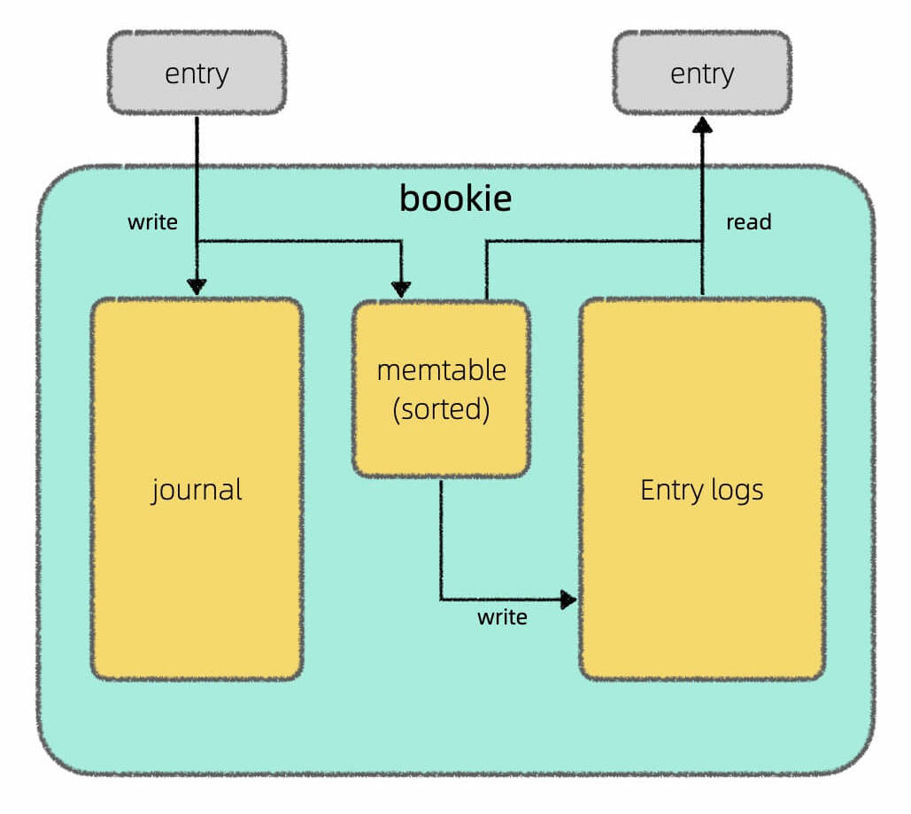
In this diagram, Journal is the same as log, and Entry Log is a group of SSTables. They just have different names.

A memtable is an in-memory ordered data structure like a red-black tree or skip list. It helps with caching and sorting new data by key. When the memtable reaches a certain size, it is turned into an SSTable and written to disk for persistent storage.

A SSTable (Sorted String Table) is simply a specially formatted file where the data is sorted by key. You can think of it like a sorted array. An LSM tree is a collection of multiple SSTables.

A log file records the operation logs. When data is written to the memtable, it is also written to the log on disk at the same time. The purpose is for data recovery. For example, if the data in the memtable hasn’t been written to an SSTable yet and there’s a sudden power failure, all the data in the memtable would be lost. But, because of the log file, this data can be recovered. After the data in the memtable is safely written as an SSTable, the related logs can be deleted.

The write process (set) of LSM tree is simple: write to both log and memtable, and finally turn the data into an SSTable and persist it on disk.

The key part is the read and compact process: How should SSTables be organized so we can quickly get the value for a key? How do we periodically compact and clean up the SSTables?

There are several ways to do this. A common way is to organize SSTables in levels:

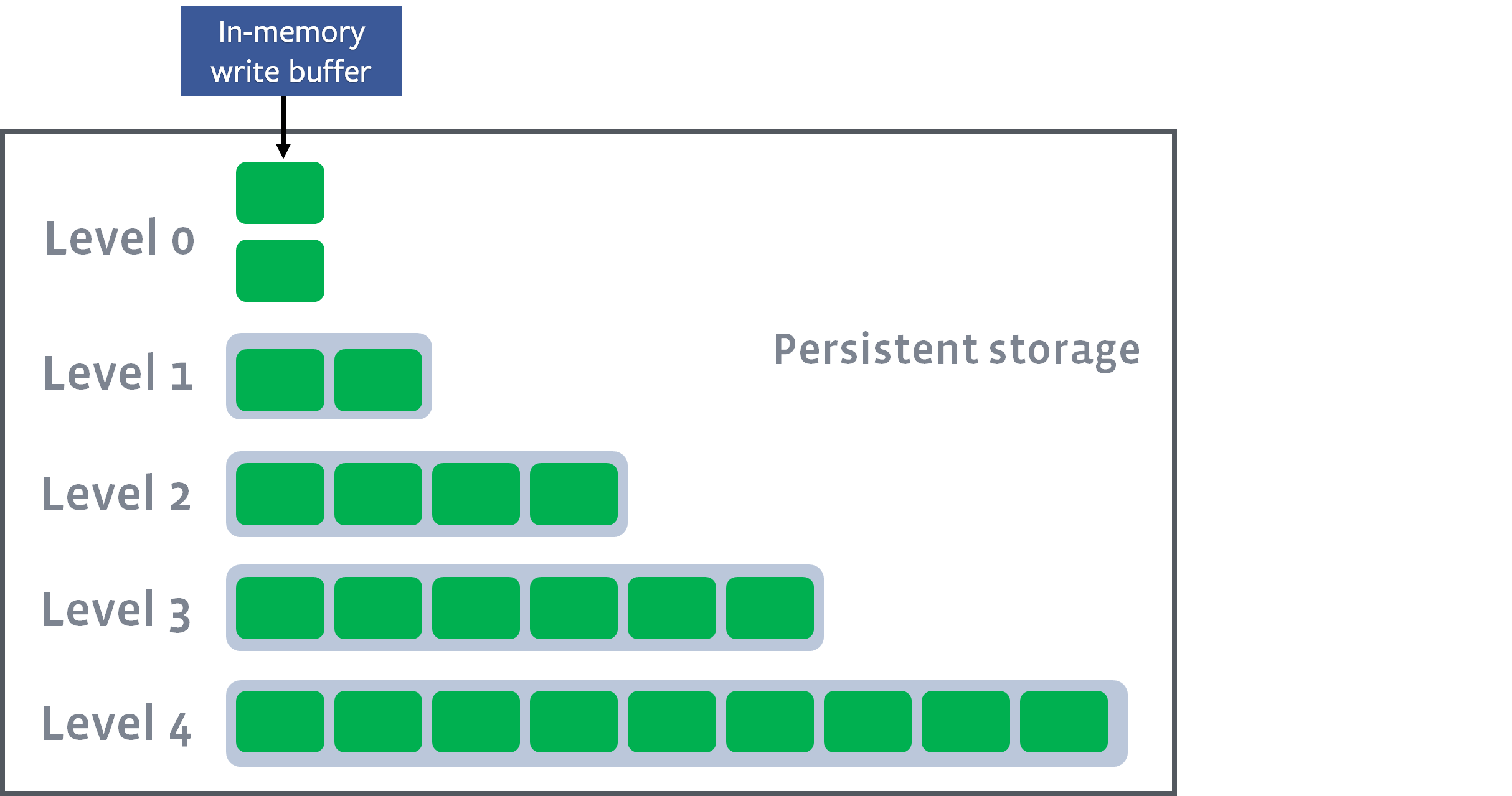
In this figure, each green block is an SSTable. Several SSTables form a level, and there are several levels. Each level can hold more SSTables as you go down.

New SSTables go into Level 0. If the number of SSTables in any level is over the limit, a compact operation is triggered. Some SSTables from this level and the next are picked based on key ranges and merged into a larger SSTable, which goes to the next lower level:

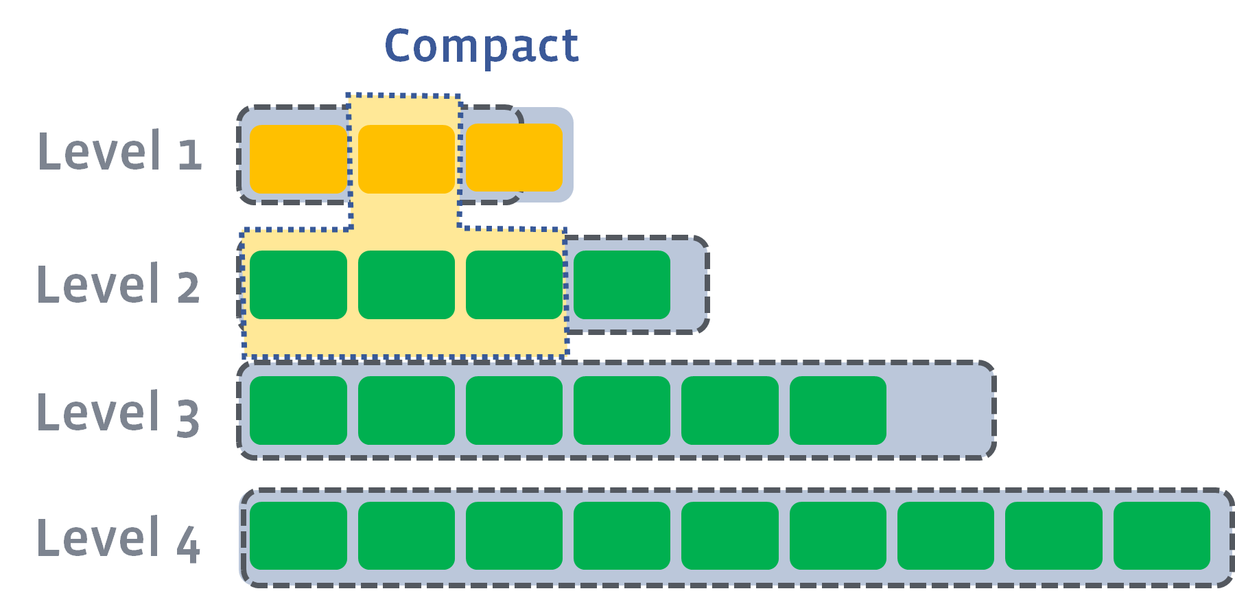
Each SSTable is like a sorted array or linked list. Merging multiple SSTables is like merging multiple sorted linked lists, as described in Linked List Double Pointer Tricks.

So, data in the upper levels is newer, and data in the lower levels is older. The algorithm ensures that the key ranges of different SSTables in the same level do not overlap:

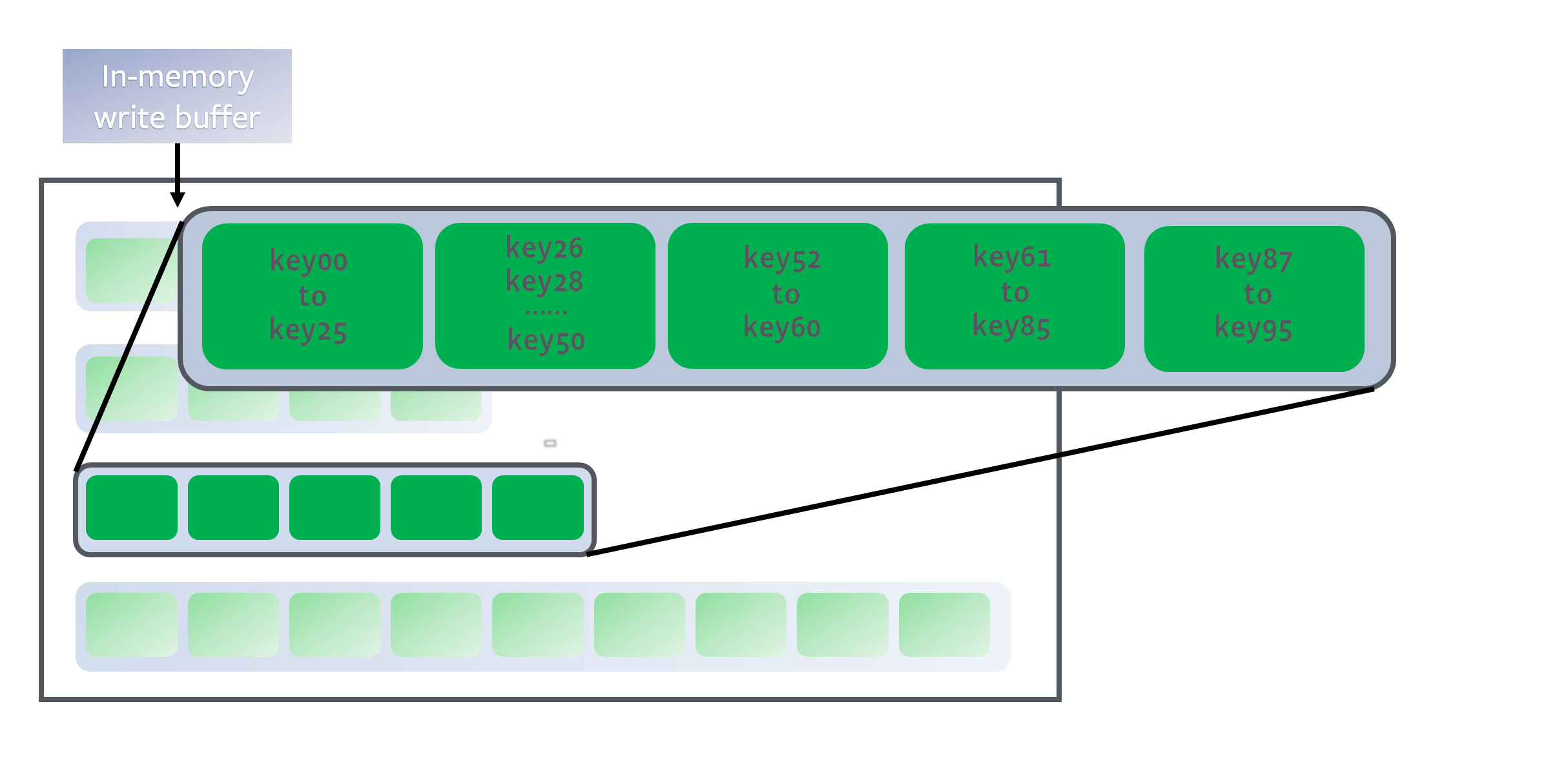
Suppose we are looking for a target key key27. We only need to scan from top to bottom, and for each level, use binary search to find the SSTable whose key range contains key27. Then, we use a Bloom filter to quickly check if key27 might exist in this SSTable.

If so, since the keys in each SSTable are sorted, we can use binary search again to find the value for the key.

This way, by using the LSM tree’s level structure and the order of keys in each SSTable, we can use binary search to speed up lookups and avoid linear search.