Algorithm Visualization Introduction

Basic Usage

The left side is the code panel, where the currently executed code line is highlighted. You can click on the code to run it to a specific position; hovering your mouse over the code for 0.5 seconds allows you to jump to the previous or next execution position.

The top contains control buttons and sliders that allow you to finely control the code's step-by-step execution. The edit button lets you modify and run my preset code.

The right side is the visualization area, displaying variables, data structures, stack information, recursion trees, etc. Hovering over data structures reveals detailed information.

The bottom left corner is the Log Console, where the output content from console.log in your code will be displayed.

The bottom right corner has floating buttons providing functions such as copying code, copying links, refreshing the panel, full-screen display, and showing/hiding the Log Console. If you find the embedded panel too small, click the full-screen button for a better view.

Understanding these features is enough for you to explore the visualization panel. Try out these features briefly below.

The content above is sufficient for beginners. The following content introduces special features of the visualization panel for interested readers.

Visualization of Data Structures

The panel can visualize common data structures such as arrays, linked lists, binary trees, hash tables, and hash sets. Below is a detailed introduction on how to create these data structures.

Standard Library Data Structures

For JavaScript's built-in data structures like arrays and hash tables, simply initialize and operate them as usual, for example:

Singly Linked List

Let's first talk about singly linked lists. Each node in a singly linked list has val and next attributes, which are exactly the same as the definition used on LeetCode.

// Singly linked list node
abstract class ListNode {
    val: any
    next: ListNode | null

    constructor(val: any, next: ListNode | null = null) {
        this.val = val
        this.next = next
    }
}

abstract class LinkedList {
    // Create a linked list and return the head node
    static createHead(elems: any[]): ListNode {
        
    }

    // Create a linked list with a cycle and return the head node
    static createCyclicHead(elems: any[], index: number): ListNode {
        
    }
}

Doubly Linked List

Each node in a doubly linked list has val, prev, and next properties, with a constructor identical to that used in LeetCode.

// Double linked list node
abstract class DListNode {
    next: DListNode | null = null
    prev: DListNode | null = null
    val: any

    constructor(val: any = 0, prev: DListNode = null, next: DListNode = null) {
        this.val = val
        this.prev = prev
        this.next = next
    }
}

// Double linked list
abstract class DLinkedList {
    // Create a double linked list and return the head node
    static createHead(elems: any[]): DListNode {
        
    }
}

Hash Table Based on Chaining

The JavaScript standard library provides a Map for storing key-value pairs. The hash table provided here is mainly for educational purposes, to accompany Principles and Implementation of Hash Tables.

The ChainingHashMap.create method can create a simplified hash table based on chaining, which only supports storing integer key-value pairs and does not support resizing. For specific implementation details, refer to Hash Table Implementation Using Chaining.

// A simplified version of chaining hash map
abstract class ChainingHashMap {

    // Create a chaining hash map with capacity
    static create(capacity: number): ChainingHashMap {
        
    }

    // Add or Update key-value pair
    abstract put(key: number, value: number): void;

    // Get the value of a key, return -1 if not found
    abstract get(key: number): number;

    // Remove a key-value pair
    abstract remove(key: number): void;

    // Get the internal array
    abstract getTable(): Array<ListNode | null>;

    // Get the head node of the linked list at a given
    abstract getTableIndex(index: number): ListNode | null;
}

Hash Table Based on Linear Probing

Similar to the chaining method, the hash table based on linear probing is also designed for teaching purposes to complement the article Principles and Implementation of Hash Tables.

The LinearProbingHashMap.create method can create a simplified hash table based on linear probing. It only supports storing integer key-value pairs and does not support resizing. For detailed implementation, you can refer to Implementing Hash Tables with Linear Probing.

// A simplified version of linear probing hash map
abstract class LinearProbingHashMap {

    // Create a linear probing hash map with capacity
    static create(capacity: number): LinearProbingHashMap {
        
    }

    // Add or Update key-value pair
    abstract put(key: number, value: number): void;

    // Get the value of a key, return -1 if not found
    abstract get(key: number): number;

    // Remove a key-value pair
    abstract remove(key: number): void;

    // Get the internal array
    abstract getTable(): Array<string | null>;
}

Binary Tree

Each node in a binary tree has the properties val, left, right, consistent with the constructor in LeetCode.

You can quickly create a binary tree using the BTree.create method. Note that we use a list to represent the binary tree, in the same way as the representation of binary trees in LeetCode problems.

// Binary Tree Node
abstract class TreeNode {
    val: any
    left: TreeNode | null
    right: TreeNode | null

    constructor(val: any, left: TreeNode | null = null, right: TreeNode | null = null) {
        this.val = val
        this.left = left
        this.right = right
    }
}

abstract class BTree {

    // Create a binary tree root node from an array in the format of LeetCode
    static createRoot(elems: any[]): TreeNode {
        
    }

    // Create a BST from a list of elements, return the root node
    static createBSTRoot(elems: number[]): TreeNode {
        
    }
}

N-ary Tree

Each node in an N-ary tree has val and children attributes, with the constructor being identical to the one used in LeetCode.

// N-ary tree node
abstract class NTreeNode {
    val: any
    children: NTreeNode[]
}

abstract class NTree {
    // Create an N-ary tree from an array
    // The input format is similar to this LeetCode problem:
    // https://leetcode.com/problems/n-ary-tree-level-order-traversal/
    static create(items: any[]) {
        
    }
}

Standard Binary Search Tree

You can use BSTMap.create to create a standard binary search tree for storing key-value pairs. For the underlying principles, refer to Implementing TreeMap/TreeSet.

If you do not need to store key-value pairs, you can use BTree.createBSTRoot mentioned above to create a binary search tree based on standard binary tree nodes.

type compareFn = (a: any, b: any) => number

const defaultCompare = (a: any, b: any) => {
    if (a === b) return 0
    return a < b ? -1 : 1
}

abstract class BSTNode {
    abstract key: any
    abstract value: any

    abstract left: null | BSTNode
    abstract right: null | BSTNode
}

abstract class BSTMap {
    static create(elems: any[] = [], compare: compareFn = defaultCompare): BSTMap {
    }

    abstract get(key: any): any

    abstract containsKey(key: any): boolean

    abstract put(key: any, value: any): void

    abstract remove(key: any): void

    abstract getMinKey(): any | null

    abstract getMaxKey(): any | null

    abstract keys(): any[]

    abstract _getRoot(): BSTNode | null
}

Red-Black Binary Search Tree

You can create a red-black binary search tree to store key-value pairs using the RBTreeMap class. For usage examples, refer to Red-Black Tree Basics.

type compareFn = (a: any, b: any) => number

const defaultCompare = (a: any, b: any) => {
    if (a === b) return 0
    return a < b ? -1 : 1
}

// Red-Black Tree Node
abstract class RBTreeNode {
    // Node color
    static RED: string = '#b10000'
    static BLACK: string = '#464546'

    abstract key: any
    abstract value: any

    abstract color: string

    abstract left: null | RBTreeNode
    abstract right: null | RBTreeNode


    static isRed(node: RBTreeNode): boolean {
        if (!node) return false
        return node.color === RBTreeNode.RED
    }

}

abstract class RBTreeMap {
    static create(elems: any[][] = [], compare: compareFn = defaultCompare): RBTreeMap {
    }

    abstract put(key: any, value: any): void

    abstract get(key: any): any

    abstract containsKey(key: any): boolean

    abstract getMinKey(): any | null

    abstract getMaxKey(): any | null

    abstract deleteMinKey(): void

    abstract deleteMaxKey(): void

    abstract delete(key: any): void

    abstract keys(): any[]

    abstract _getRoot(): RBTreeNode | null

    // Some key methods of Red-Black Tree
    static makeNode(key: any, value: any, color: string): RBTreeNode {
    }

    static makeRedNode(key: any, value: any): RBTreeNode {
    }
    
    static makeBlackNode(key: any, value: any): RBTreeNode {
    }

    // Left rotation operation
    static rotateLeft(node: RBTreeNode): RBTreeNode {
    }
    
    static moveRedLeft(node: RBTreeNode): RBTreeNode {
    }
    
    // Right rotation operation
    static rotateRight(node: RBTreeNode): RBTreeNode {
    }
    
    static moveRedRight(node: RBTreeNode): RBTreeNode {
    }
    
    // Color flip
    static flipColors(node: RBTreeNode): void {
    }

    // Balance operation
    static balance(node: RBTreeNode): RBTreeNode {
    }
}

Binary Heap (Priority Queue)

In Binary Heap Basics and Implementation, I explained the fundamental concepts of binary heaps, the code implementation of priority queues, and the two core operations: swimming (swim) and sinking (sink), using a visual panel. Additionally, some methods of binary heaps are also used in Heap Sort Algorithm Details to perform sorting.

type compareFn = (a: any, b: any) => number

const defaultCompare: compareFn = (a, b) => {
    if (a < b) return -1;
    if (a > b) return 1;
    return 0;
};

// Binary heap node
abstract class HeapNode {
    abstract val: any;
    abstract left: HeapNode;
    abstract right: HeapNode;
}

abstract class Heap {

    // Create a heap, you can pass in initial elements or a comparison function
    static create(items: any[] = [], fn: compareFn = defaultCompare): Heap {
        
    }

    // Create a max heap, you can pass in initial elements
    static createMax(items?: any[]): Heap {
        
    }

    // Create a min heap, you can pass in initial elements
    static createMin(items?: any[]): Heap {
        
    }

    // Create a binary heap node
    static makeNode(value: any): HeapNode {
        
    }

    // Add an element to the top of the heap
    abstract push(value: any): void;

    // Pop the top element of the heap
    abstract pop(): any;

    // View the top element of the heap
    abstract peek(): any;

    // Get the number of elements in the heap
    abstract size(): number;

    // Display the underlying array
    abstract showArray(varName?: string): any[];

    // Return the root node of the heap
    // Mainly used to explain the principle of binary
    abstract _getRoot(): HeapNode | null;

    // Convert an array to a complete binary tree, but will not apply the properties of heap
    // Mainly used to explain heap sort
    static init(items: any[], fn: compareFn = defaultCompare) {
        
    }

    // Make the node swim up and maintain the properties of the binary heap
    // Mainly used to explain heap sort
    static sink(heap: Heap, topIndex: number, size: number, compare: compareFn) {
        
    }

    // Make the node sink and maintain the properties of the binary heap
    // Mainly used to explain heap sort
    static swim(heap: Heap, index: number, compare: compareFn) {
        
    }
}

The visualization panel by default displays a binary heap in the logical structure of a binary tree. By calling the showArray method, you can simultaneously display the underlying array structure of the binary heap. Below are some examples of usage:

Segment Tree

The SegmentTree class allows for the creation of segment trees and supports methods such as query and update. The underlying principles can be found in Introduction to Segment Trees.

Currently, built-in segment trees for sum, maximum, and minimum values are available. You can directly use the SegmentTree.create method to create a custom segment tree.

type mergeFn = (a: any, b: any) => any

const sumMerger = (a: any, b: any) => a + b
const maxMerger = (a: any, b: any) => Math.max(a, b)
const minMerger = (a: any, b: any) => Math.min(a, b)

// Segment tree node
abstract class SegmentNode {
    abstract val: any
    abstract l: number
    abstract r: number

    abstract left: SegmentNode | null
    abstract right: SegmentNode | null
}

// Segment tree
abstract class SegmentTree {

    // Create a custom segment tree
    // merger is a function that defines the merge logic of the segment tree
    // mergerName is the name of the merge rule, to display on visualization panel
    static create(items: any[], merger: mergeFn = sumMerger, mergerName: string = 'sum'): SegmentTree {
    }

    // Create a sum segment tree, supports range sum query and single update
    static createSum(items: any[]): SegmentTree {
        return SegmentTree.create(items, sumMerger, 'sum')
    }

    // Create a min segment tree, supports range min query and single update
    static createMin(items: any[]): SegmentTree {
        return SegmentTree.create(items, minMerger, 'min')
    }

    // Create a max segment tree, supports range max query and single update
    static createMax(items: any[]): SegmentTree {
        return SegmentTree.create(items, maxMerger, 'max')
    }

    // Update the value at index to value
    abstract update(index: number, value: any): void

    // Query the value of the closed interval [left, right]
    abstract query(left: number, right: number): any

    // Show the underlying array
    abstract showArray(varName: string): any[]

    // Get the root node of the segment tree
    abstract _getRoot(): SegmentNode | null
}

The visualization panel below creates a segment tree for summation, displaying the logical structure of the segment tree, the underlying array, and basic operations such as query and update:

Graph Structures

In the article Fundamentals and General Implementations of Graph Structures, I discussed how the logical structure of graphs is similar to multi-way trees and can be represented using Vertex and Edge classes for vertices and edges. However, in practice, when implementing graph structures in code, we typically use adjacency lists or adjacency matrices.

The visualization panel also implements a Graph class to create graph structures, supporting weighted/unweighted and directed/undirected graphs. For educational purposes, the Graph class in the visualization panel maintains three implementation methods: adjacency lists, adjacency matrices, and the Vertex, Edge classes.

Here is an example using DFS to find all paths from node 0 to node 4 in a graph. You can click the line if (s === n - 1) multiple times to observe the graph traversal process:

// Adjacency list structure type
type AdjacencyList = {
    // key is the vertex id
    // value is an array, storing information of neighbor nodes
    // If it is an unweighted graph, the array element is a number, representing
    // If it is a weighted graph, the array element is an array, the first
    // element is the node id, the second element is the weight of the edge
    [key: number]: (number | [number, number])[];
};

abstract class Graph {
    // Create a directed graph from multiple edges
    // Each element in edges is an array representing a directed edge
    // The first element is the start vertex id, the second element is the end vertex id
    // If there is a third element, it represents the weight of the edge
    // If there is no third element, the graph is unweighted
    static createDirectedGraphFromEdges(edges: any[][]): Graph {
    }

    // Create an undirected graph from multiple edges
    // The input format is similar to
    // createDirectedGraphFromEdges, except that the
    static createUndirectedGraphFromEdges(items: any[][]): Graph {
    }

    // Create a directed graph from adjacency list
    // adjList is an array, each element is an array representing the neighbors of a vertex
    // If the neighbor is a number, it represents an unweighted edge
    // Example:
    // Graph.createDirectedGraphFromAdjList([
    //   [1], [2], [0]
    // ])
    // A directed graph with three vertices, three edges are 0 -> 1, 1 -> 2, 2 -> 0
    // If the neighbor is an array, the first element is the
    // end vertex id, the second element is the weight of the
    // Example:
    // Graph.createDirectedGraphFromAdjList([
    //   [[1, 9]],
    //   [[2, 8]],
    //   [[0, 5]]
    // ])
    // A directed graph with three vertices, three edges are
    // 0 -> 1, 1 -> 2, 2 -> 0, with weights 9, 8, 5
    static createDirectedGraphFromAdjList(adjList: (number | [number, number])[][]): Graph {
    }

    // Create an undirected graph from adjacency list
    // The input format is similar to
    // createDirectedGraphFromAdjList, except that the
    static createUndirectedGraphFromAdjList(adjList: (number | [number, number])[][]): Graph {
    }

    // Get the neighbor node id of the node
    abstract neighbors(id: number): number[]

    // Get the weight of the edge from->to
    // If it is an unweighted graph, the default return is 1
    abstract weight(from: number, to: number): number

    // Get the number of vertices
    abstract length(): number

    // Return the adjacency list structure
    abstract getAdjList(): AdjacencyList

    // Return the adjacency matrix structure
    abstract getAdjMatrix(): number[][]

    // Get the vertex object by id, only used for visualization coloring
    abstract _v(id: number): Vertex

    // Get the from->to Edge object, only used for visualization coloring
    abstract _e(from: number, to: number): Edge

}

// Vertex object
abstract class Vertex {
    id: any
}

// Edge object
abstract class Edge {
    from: Vertex
    to: Vertex
    weight: number
}

Union-Find

The UF class can create a union-find structure, which is used to solve dynamic connectivity problems in graph structures. The underlying principles can be found in Core Principles of Union-Find.

Since the union-find structure can be optimized in various ways, such as path compression and weighted union, the UF class offers multiple initialization methods:

• UF.createNative(n: number): Creates an unoptimized union-find structure with n nodes.
• UF.createWeighted(n: number): Creates a union-find structure optimized with a weight array, containing n nodes.
• UF.createPathCompression(n: number): Creates a union-find structure optimized with path compression, containing n nodes.

The UF object mainly provides the following three methods to solve dynamic connectivity problems:

• union(p: number, q: number): Merges the connected components containing nodes p and q.
• connected(p: number, q: number): Determines if nodes p and q are in the same connected component.
• count(): Returns the number of connected components in the current union-find structure.

The logical structure of a union-find is a forest (several multi-way trees). For easier visualization, a virtual node is created in this forest. The virtual node is transparent, with the root of each multi-way tree displayed in red and regular nodes in green. This allows the forest structure to be displayed as a multi-way tree while making it easy to see the root of each connected component.

The union-find is implemented using an array to represent the forest. By calling the showArray method, the visualization panel can simultaneously display this underlying array.

Below is an example of a union-find optimized with a weight array:

abstract class UF {
    
    // Create a naive union-find with size n
    static createNaive(n: number): UF {
        
    }

    // Create a weighted union-find with size n
    static createWeighted(n: number): UF {
        
    }

    // Create a path compression union-find with size n
    static createPathCompression(n: number): UF {
        
    }

    // Create a union-find with size n, default to path compression
    static create(n: number): UF {
        return UF.createPathCompression(n)
    }

    // Find the root of p
    find(p: number): number {
        
    }

    // Merge the connected components of p and q
    union(p: number, q: number): void {
        
    }

    // Check if p and q are in the same connected component
    connected(p: number, q: number): boolean {
        
    }

    // Return the number of connected components
    count(): number {
        
    }

    // Show the parent array of the union-find
    showArray(varName: string): void {
        
    }
}

Trie Tree/Prefix Tree/Dictionary Tree

Trie.create() allows you to create a Trie tree, where blue nodes are regular Trie nodes and purple nodes are nodes that contain words. Hovering over a node will display the word stored in that node.

// Trie Node
abstract class TrieNode {
    abstract char: string
    abstract isWord: boolean
    abstract children: TrieNode[]
}

// Trie API
abstract class Trie {

    // Create a trie, words will be added to the trie
    static create(words?: string[]): Trie {
        
    }

    // Add a string to the trie
    add(word: string) {
        
    }

    // Remove a string from the trie
    remove(word: string) {
        
    }

    // Return the shortest prefix of word
    shortestPrefixOf(word: string) {
        
    }

    // Return the longest prefix of word
    longestPrefixOf(word: string) {
        
    }

    // Check if there is a string with prefix
    hasKeyWithPrefix(prefix: string) {
        
    }

    // Return all strings with prefix
    keysWithPrefix(prefix: string) {
        
    }

    // Return all strings that match the pattern
    keysWithPattern(pattern: string) {
        
    }

    // Check if the word exists in the trie
    containsKey(word: string) {
        
    }

    // Return the number of strings in the trie
    size() {
        
    }
}

Enhanced console.log

Previously, I shared a technique for debugging recursive algorithms using only standard output during exams, which involves using additional indentation to distinguish recursion depth.

To make it easier for everyone to observe the output of complex algorithms more intuitively, I enhanced the console._log function in the visualization panel.

The specific enhancements are as follows:

1. If you use the console._log function in the visualization panel, the output will be printed in the Log Console at the bottom left, with automatic indentation added based on recursion depth.

2. Clicking on the output in the console will display a dashed line that aligns all outputs with the same indentation, helping you understand which outputs belong to the same recursion depth.

The code outputs when starting and ending a recursion. You can see that the console in the bottom left displays the following output, with outputs from the same recursion depth having the same indentation for easy distinction:

enter traverse(1)
  enter traverse(2)
    enter traverse(3)
      enter traverse(4)
      leave traverse(4)
    leave traverse(3)
  leave traverse(2)
leave traverse(1)

You can click on the first character e or l of each line of output in the console to see a dashed line that aligns all outputs with the same indentation, making it easier to see the correspondence between enter and leave.

Visualization of Sorting Algorithms

The @visualize shape nums rect annotation can transform an array into a histogram-like form based on the size of its elements. This helps to intuitively understand the size relationships of array elements, facilitating the observation of the sorting algorithm's execution process. Using @visualize shape nums cycle can revert array elements to the default circular display.

Let's take Insertion Sort as an example:

Binding Variables to Array Indices

By default, when a variable name is used to access an array as an index, it automatically binds to the array, displaying a cursor on the array to show the element it points to. However, sometimes a variable may not access array elements directly, yet we still want it to be displayed on the array.

For example, in the insertion sort visualization mentioned above, the sortedIndex variable never appears in the code as an array access like nums[sortedIndex]. Nevertheless, we want the sortedIndex variable to be displayed in the visualization panel on the right, as it marks the boundary between sorted and unsorted elements.

In this case, we can use the @visualize bind nums[sortedIndex] annotation to bind the sortedIndex variable to the nums array. This way, a cursor will continuously display the position of sortedIndex on the right-side nums array.

To unbind, you can use the @visualize unbind nums[sortedIndex] annotation.

Color System

You can set the color of nodes/elements using the @visualize color annotation. The color is a hex color code starting with #, such as #8ec7dd for light blue.

The color code can include ?, representing a random hexadecimal number, to generate random colors, like #8e??dd.

For instance, in the insertion sort visualization above, I used @visualize color nums[sortedIndex] #8ec7dd to set the color of the sortedIndex variable. The array element pointed to by sortedIndex will turn light blue, and when the sortedIndex variable moves to a new index, the old index's element will revert to the default color.

If you wish to color a specific array index without it changing as the variable moves, use * to mark it as a fixed element color.

For example, @visualize color *nums[0] #8ec7dd or @visualize color *nums[sortedIndex] #8ec7dd. When sortedIndex = 2, nums[2] will turn light blue, and nums[2] will remain light blue regardless of changes in sortedIndex.

This applies similarly to node objects. You can color variables, like @visualize color root #8ec7dd, or specific nodes, like @visualize color *root.left #8ec7dd.

To remove a color setting, use #unset as the color code, such as @visualize color *root.left #unset, to revert to the default color.

After setting colors with the @visualize color annotation, the color code will appear as a color picker, allowing you to click and modify the color.

Variable Hiding and Scope Elevation

Use @visualize global to elevate a variable's scope to global, allowing closure variables to remain visible in the right-side visualization panel.

Use @visualize hide to hide variables, helping to keep the right-side visualization panel from becoming too cluttered.

Here is an example illustrating the use of these annotations. Suppose I want to implement a simple Stack class with push, pop, and peek methods using JavaScript function closures:

At the final step, you can see the stack variable persistently appears as an Object in the right-side visualization panel, occupying significant space without practical meaning.

We are actually more interested in the items variable, as observing the changes in this array helps us understand how the push and pop methods work.

However, since items is declared inside the Stack function, it is not in the current scope when the code executes outside the function body, so it won't be visualized on the right panel.

In this case, we can use the @visualize global annotation to elevate the items variable to the global scope and use the @visualize hide annotation to hide the stack variable in the right panel.

This achieves our desired outcome. Please click on the stack.push(1); line of code and proceed to execute it. You'll see that the stack variable no longer appears, and the update process of the items array is displayed on the right side:

Visualization of Backtracking/DFS Recursive Process

Recursive algorithms can be challenging for many readers. I previously wrote an article, Understanding All Recursive Algorithms from a Tree Perspective, which abstractly outlines the fundamental thinking model and writing techniques for recursive algorithms.

In simple terms: Consider the recursive function as a pointer on a recursive tree. Backtracking algorithms traverse a multi-branch tree and collect the values of the leaf nodes; dynamic programming involves decomposing a problem and using the solutions of subproblems to derive the solution of the original problem.

Now, I have integrated the thinking model discussed in the article into an algorithm visualization panel, which will surely help you understand the execution process of recursive algorithms more intuitively.

For recursive algorithms, the annotations @visualize status, @visualize choose, and @visualize unchoose can be very helpful. Below, I will introduce them one by one.

Example of @visualize status

In short, the @visualize status annotation can be placed above a recursive function that needs visualization, to control the values of nodes in the recursion tree.

Let's take a simple example. When explaining the Core Framework of Dynamic Programming Algorithms, I illustrated the recursion tree for the Fibonacci problem, where larger problems at the top are gradually decomposed:

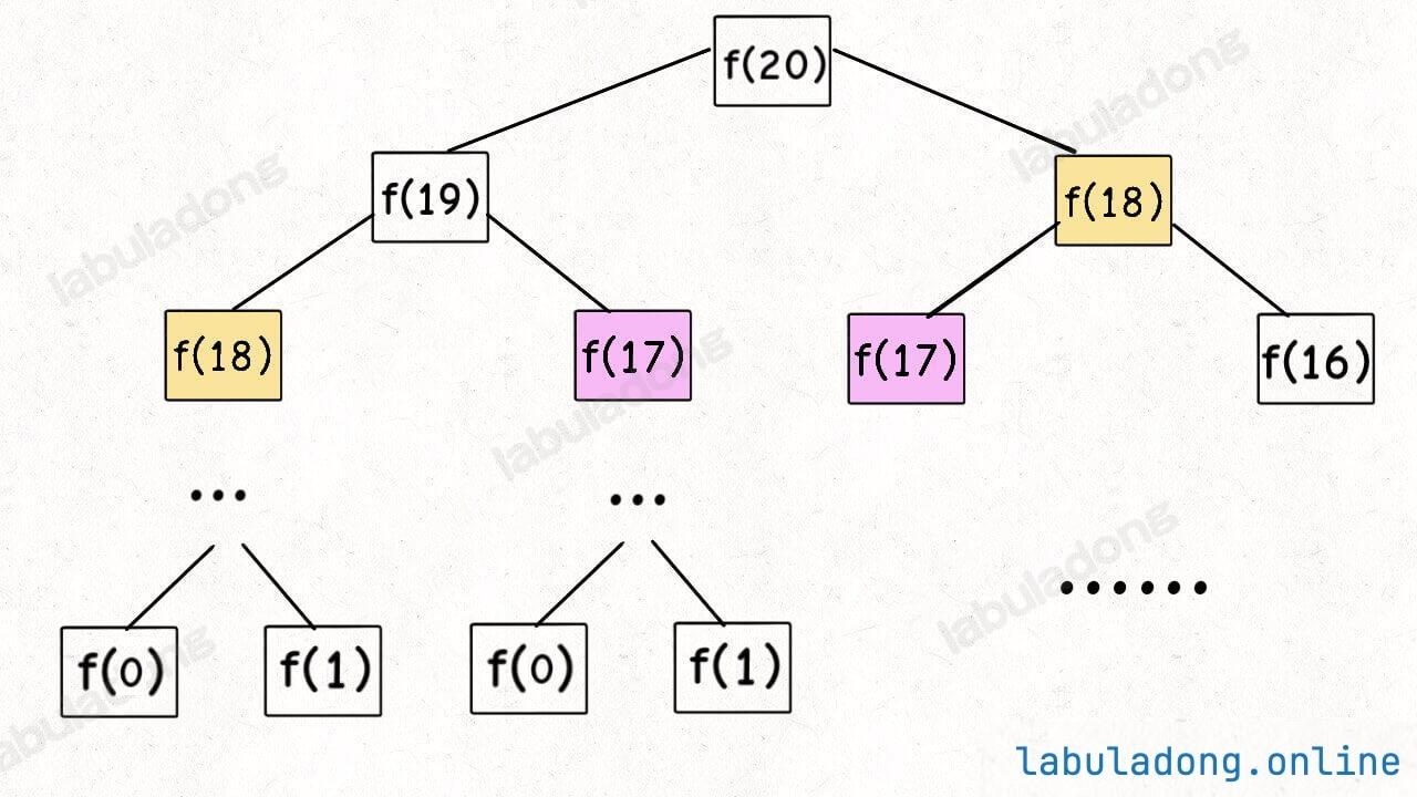
How do we describe the process of an algorithm running? The recursive function fib acts like a pointer on the recursion tree, repeatedly decomposing the original problem into subproblems. When the problem is broken down to a base case (leaf node), it starts returning the answers of subproblems layer by layer, deriving the answer to the original problem.

With the @visualize status annotation, this process can be seen clearly. The panel below shows the recursion tree of the Fibonacci algorithm, attempting to compute the value of fib(3):

The @visualize status annotation placed above the fib function means:

1. It enables the recursion tree visualization for this fib function, with each recursive call visualized as a node on the recursion tree. The value of n in the function parameters is displayed as the state on the node.

2. The fib function is seen as a pointer traversing this recursion tree, with branches along the stack path highlighted.

3. If the function has a return value, once the function ends and a return value for a node is calculated, hovering the mouse over this node will display the return value.

The previously shown Fibonacci solution code did not include memoization, resulting in an exponential time complexity. Now, let's experience how adding memoization affects the growth of the recursion tree.

By visualizing the entire tree this way, you can intuitively understand how dynamic programming uses memoization to eliminate overlapping subproblems.

@visualize choose/unchoose Example

In short, the @visualize choose/unchoose annotations are placed before and after the recursive function calls, respectively, to control the values on the branches of the recursion tree.

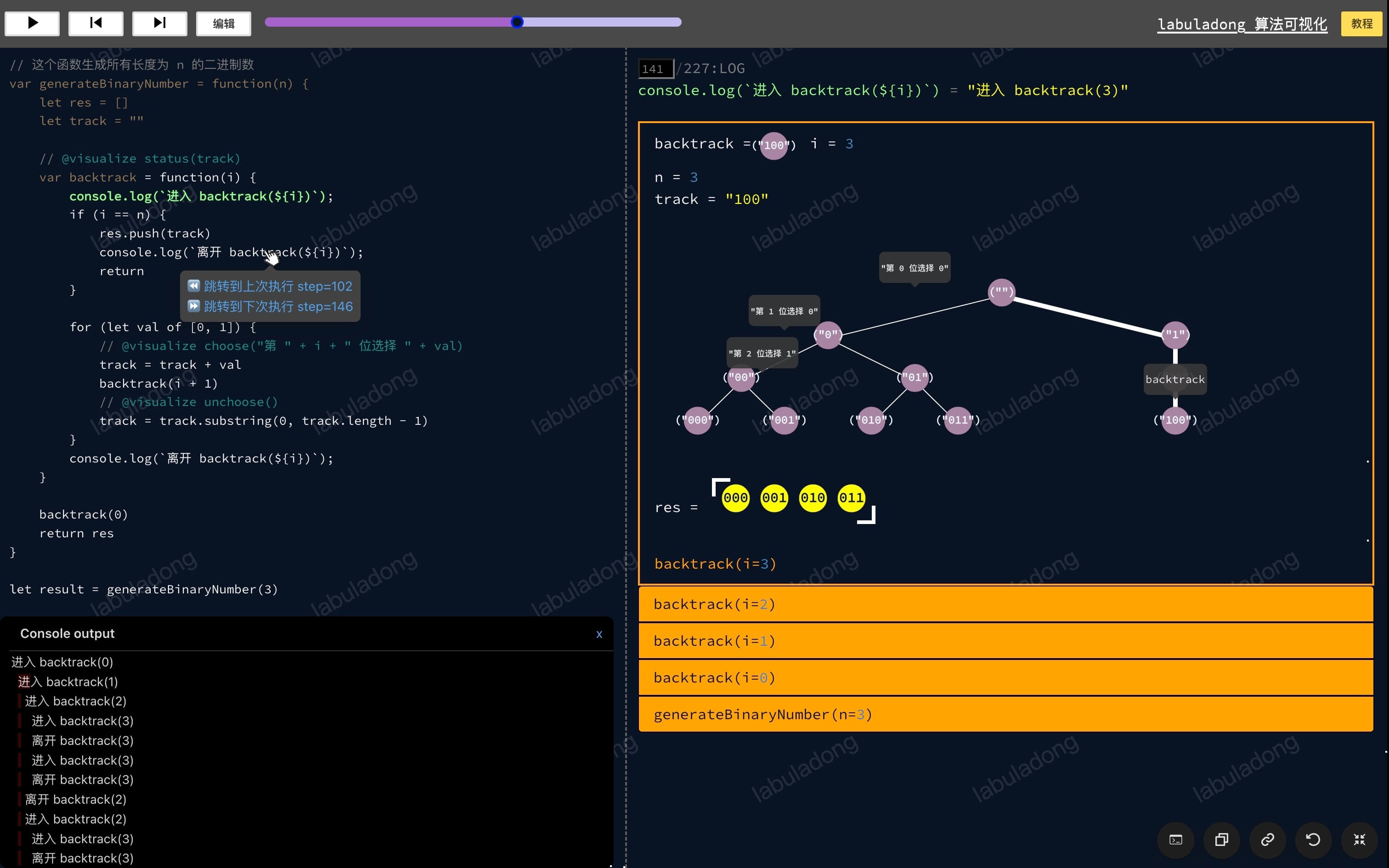
Let me illustrate with a simple backtracking problem. For instance, you need to write a generateBinaryNumber function that generates binary numbers of length n. For example, when n = 3, the function should generate 000, 001, 010, 011, 100, 101, 110, 111, which are the 8 binary numbers.

The solution code for this problem isn't complex. I'll demonstrate how to use the @visualize choose/unchoose annotations to visualize the backtracking process:

You can hover your mouse over any node in the recursion tree to display all the information on the path from the root node to that node.

Understanding the recursion algorithm code in conjunction with this recursion tree makes it quite intuitive, doesn't it?

BFS Process Visualization

As mentioned in Binary Tree Thinking (Overview), the BFS algorithm is an extension of the level-order traversal of a binary tree.

Since recursion trees can be visualized, the BFS process can also be visualized. You can use @visualize bfs to enable the automatic visualization of the BFS algorithm, generating a brute-force tree. The values on the nodes represent the values of elements in the queue, and with @visualize choose/unchoose annotations, you can control the values on the branches.

Below, I will demonstrate the visualization of the BFS process with a simple example:

Scenario Practice Questions

Below, I will present specific algorithmic problems and ask you questions, requiring you to efficiently analyze the problems and algorithms using the visualization panel. I will provide answers, allowing you to think through the problems first before seeing my solutions.

This section primarily utilizes the "Execute to Specified Code Location" feature of the visualization panel: you can click on a specific part of the code, and the algorithm will execute up to that point, visualizing the process. Using this feature effectively can significantly enhance your understanding of algorithms.

Warm-Up

First, let's familiarize ourselves with the "Execute to Specified Code Location" feature. In the previously demonstrated single linked list cycle detection algorithm, I had you repeatedly click on the line if (slow === fast) to observe the chasing process of the fast and slow pointers:

Why does clicking this part show the chasing process of the fast and slow pointers? Because at this point in the execution, the fast and slow pointers have just moved, allowing you to see their complete movement process.

Scenario One: Preorder, Inorder, and Postorder Traversal of a Binary Tree

Scenario Two: Observing the Growth of the Recursive Tree

Scenario Three: Quickly Obtain a Brute-Force Result

Scenario Four: Understanding Top-Down and Bottom-Up Thinking Patterns