Time and Space Complexity Analysis Practical Guide

My previous articles primarily focused on explaining algorithm principles and problem-solving thinking, often glossing over the analysis of time and space complexity for the following reasons:

1. For beginner readers, I want you to concentrate on understanding the principles of algorithms. Adding too much mathematical content can easily discourage readers.

2. A correct understanding of the underlying principles of common algorithms is a prerequisite for analyzing complexity. Especially for recursion-related algorithms, only by thinking and analyzing from a tree perspective can you correctly analyze their complexity.

Since historical articles now cover the core principles of all common algorithms, I have specifically written a guide on time and space complexity analysis. Instead of giving you a fish, it is better to teach you how to fish by providing a general method to analyze the time and space complexity of any algorithm.

This article will be lengthy and cover the following points:

1. Using time complexity to deduce problem-solving approaches, reducing trial and error.

2. Where does the time go? Common coding mistakes that lead to algorithm timeouts.

3. Basic characteristics of Big O notation.

4. Analysis of time complexity in non-recursive algorithms.

5. Efficiency measurement methods of data structure APIs (amortized analysis).

6. Analysis methods for time/space complexity of recursive algorithms, with a focus on this area, using dynamic programming and backtracking algorithms as examples.

Before explaining the concept of complexity and specific calculation methods, I will discuss some common techniques and pitfalls encountered in practice.

Inferring Solution Strategies from Complexity

For example, if a problem provides an input array with a length up to 10^6, we can infer that the time complexity should be less than $O(N^2)$. It needs to be optimized to $O(NlogN)$ or $O(N)$. An algorithm with $O(N^2)$ complexity would reach about 10^12, which most judging systems cannot handle efficiently.

To keep the complexity within $O(NlogN)$ or $O(N)$, our options become limited. Suitable approaches might include sorting the array, prefix sums, two-pointer techniques, or one-dimensional dynamic programming. Starting with these strategies is more reliable. Nested for loops, two-dimensional dynamic programming, and backtracking can typically be ruled out immediately.

Another clear example is when the data scale is very small, such as an array length N not exceeding 20. In this case, we can be fairly certain that a brute-force exhaustive search is likely required.

Judging platforms tend to challenge you with larger data scales, so if they provide small data scales, it's likely because the optimal solution involves exponential or factorial complexity. You can confidently use backtracking algorithms without considering other approaches.

Therefore, it's important to consider all the information given in the problem, particularly the data scale, before starting to code. Ignoring this and diving directly into coding can lead to unnecessary detours.

Complexity Issues Due to Coding Errors

This section summarizes common coding errors, especially among beginners, that can lead to unexpected time consumption, slow down your algorithm, or even cause timeouts.

Using Standard Output

While solving algorithm problems, we might use print/console.log functions to print some states for debugging purposes.

However, remember to comment out these output statements before submitting your code, as standard output involves I/O operations that can significantly slow down your algorithm.

Incorrectly Passing by Value Instead of Reference

For example, in C++, function parameters are passed by value by default. If you pass a vector as a parameter, the data structure is fully copied, leading to additional time and space consumption. This is particularly problematic for recursive functions, where passing by value almost guarantees timeout or memory overflow.

The correct approach is to pass by reference, such as vector<int>&, to avoid unnecessary copying. Readers using other languages should verify if similar issues exist and understand their programming language's parameter passing mechanism.

Unclear Underlying Implementation of Interface Objects

This is a rather tricky problem, often occurring in object-oriented languages like Java, though it is rare. Nonetheless, it merits attention.

In Java, List is an interface with many implementing classes, such as ArrayList and LinkedList. If you have learned from the basic knowledge sections Implementing Dynamic Arrays Step by Step and Implementing Doubly Linked Lists Step by Step, you know that methods of ArrayList and LinkedList differ in complexity, such as the get method in ArrayList being $O(1)$ and in LinkedList being $O(N)$.

So, if a function parameter is passed to you as a List type, would you dare to perform list.get(i) for random access? Probably not.

In such cases, it is generally safer to create an ArrayList yourself, copy all elements from the passed List, and then access them via an index.

These are the main non-algorithmic issues to watch out for. Pay attention to them, and you should be fine. Let's move on to the formal explanation of algorithm complexity analysis.

Big O Notation

The symbol O (uppercase letter 'O', not the number 0) is commonly used to represent a set of functions. For example, $O(n^2)$ represents a set of functions derived from g(n) = n^2. When we say an algorithm has a time complexity of $O(n^2)$, it means the complexity of the algorithm is described by a function within this set.

In theory, understanding this abstract mathematical definition can answer all your questions about Big O notation.

However, since many people feel dizzy when they see mathematical definitions, I will list two properties used in complexity analysis. Remembering these two is sufficient.

1. Retain only the term with the highest growth rate; other terms can be omitted.

Firstly, constant factors in multiplication and addition can be ignored, as shown in the following example:

O(2N + 100) = O(N)
O(2^(N+1)) = O(2 * 2^N) = O(2^N)
O(M + 3N + 99) = O(M + N)

Of course, don't eliminate constants blindly. Some constants cannot be removed, as they might involve exponential rules we learned in high school:

O(2^(2N)) = O(4^N)

Besides constant factors, terms with slower growth rates can be ignored in the presence of terms with faster growth rates:

O(N^3 + 999 * N^2 + 999 * N) = O(N^3)
O((N + 1) * 2^N) = O(N * 2^N + 2^N) = O(N * 2^N)

All the examples listed above are the simplest and most common ones, which can be correctly explained by the definition of Big O notation. If you encounter more complex complexity scenarios, you can also judge whether your complexity expression is correct based on the definition.

2. Big O Notation Represents the "Upper Bound" of Complexity.

In other words, as long as you provide an upper bound, using Big O notation to represent it is correct.

For example, consider the following code:

for (int i = 0; i < N; i++) {
    print("hello world");
}

If we consider this as an algorithm, then clearly its time complexity is $O(N)$. However, if you insist on saying its time complexity is $O(N^2)$, theoretically, that's acceptable, because the O notation represents an upper bound. Indeed, the time complexity of this algorithm will not exceed the upper bound of N^2. Although this bound is not "tight," it still fits the definition, so theoretically, it's not incorrect.

The above example is too simple, and unnecessarily expanding its time complexity upper bound seems meaningless. However, some algorithms have complexities that depend on the input data, making it difficult to provide a very precise time complexity in advance. In such cases, using Big O notation to expand the upper bound of time complexity becomes meaningful.

For instance, in the previous article The Core Framework of Dynamic Programming, we discussed the brute-force recursive solution to the coin change problem. The core code framework is as follows:

// Definition: to make up the amount n, at least dp(coins, n) coins are needed
int dp(int[] coins, int amount) {
    // base case
    if (amount <= 0) return;
    // state transition
    for (int coin : coins) {
        dp(coins, amount - coin);
    }
}

When amount = 11, coins = [1,2,5], the recursive tree of the algorithm looks like this:

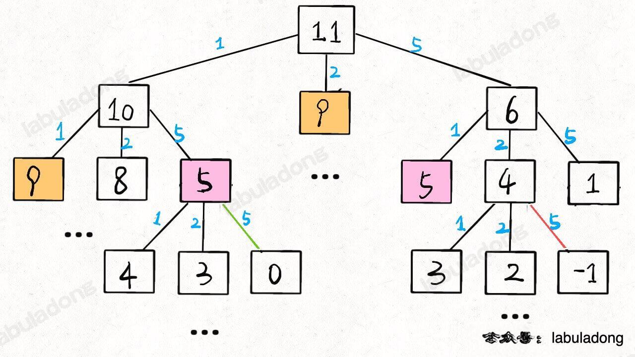
The method for calculating the time complexity of recursive algorithms will be discussed later. For now, let's determine the number of nodes in this recursive tree.

Assume the value of amount is N, and the number of elements in the coins list is K. This recursive tree is a K-ary tree. However, the growth of this tree is directly related to the denominations of coins in the coins list, resulting in an irregular structure that makes it difficult to precisely calculate the total number of nodes.

In such cases, a simpler approach is to approximate based on the worst-case scenario:

What is the height of this tree? Unknown, so we handle it based on the worst-case scenario, assuming all coins have a denomination of 1, making the tree height N.

What is the structure of this tree? Unknown, so we handle it based on the worst-case scenario, assuming it is a full K-ary tree.

How many nodes are on this tree? Handling it based on the worst-case scenario, a full K-ary tree of height N has a total number of nodes calculated using the geometric series formula (K^N - 1)/(K - 1), denoted in Big O notation as $O(K^N)$.

Of course, we know the actual number of nodes is less than this, but using $O(K^N)$ as an approximate upper bound is acceptable and clearly shows that this is an exponential algorithm that requires optimization for efficiency.

Therefore, sometimes your estimated time complexity may differ from someone else's, which doesn't necessarily mean one of you is wrong; it could simply be a difference in estimation precision.

Theoretically, we aim to achieve an accurate and "tight" upper bound, but obtaining an accurate upper bound requires strong mathematical skills. When preparing for interviews, it's acceptable to settle for less as long as the order of magnitude (linear/exponential/logarithmic/quadratic, etc.) matches.

In the field of algorithms, besides using Big O notation for asymptotic upper bounds, there are also asymptotic lower bounds and asymptotic tight bounds, which interested readers can explore on their own. However, from a practical perspective, the above explanation of Big O notation is sufficient.

Non-Recursive Algorithm Analysis

The space complexity of non-recursive algorithms is usually easy to calculate; just check if it requires arrays or similar storage space. Therefore, I will mainly discuss the analysis of time complexity.