Binary Tree Basic and Common Types

labuladongOriginalAbout 2344 words

Prerequisites

Before reading this article, you need to study:

Basics of Linked Lists (Linked Storage)

I believe the binary tree is the most important fundamental data structure, bar none.

If you are a beginner, it might be difficult for me to thoroughly explain why I arrived at this conclusion at this stage. You need to carefully study the subsequent content on this site to gradually understand. For now, I will summarize two points:

The binary tree itself is a relatively simple fundamental data structure, but many complex data structures are based on binary trees, such as Red-Black Trees (binary search trees), Multi-way Trees, Binary Heaps, Graphs, Tries, Union-Find, Segment Trees, etc. Once you master binary trees, these data structures become manageable; if you don't understand binary trees, these advanced data structures will be difficult to handle.
Binary trees not only represent a data structure but also embody a recursive mindset. All recursive algorithms, such as Backtracking Algorithms, BFS Algorithms, Dynamic Programming, essentially abstract specific problems into a tree structure. Once you abstract them, these problems ultimately revert to binary tree issues. When you look at a piece of algorithm code, it may appear as a string of text to others, but in your eyes, the code is a tree, and you can modify it correctly with ease.

The subsequent chapters on data structures contain extensive explanations and exercises on binary trees. By following the site's directory order, I will help you thoroughly understand binary trees, and then you will understand why I emphasize them so much.

Common Types of Binary Trees

The main challenge of binary trees is in solving algorithm problems; the structure itself is not difficult to understand, as it is just a tree-like structure:

Above is a simple binary tree, and here are some terms you need to know:

Nodes directly connected below a node are called child nodes, and nodes directly connected above are called parent nodes. For example, node 3's parent is 1, its left child is 5, and right child is 6. Node 5's parent is 3, its left child is 7, and it has no right child.
A tree with a child node as its root is called a subtree. For example, node 3's left subtree consists of nodes 5 and 7, and its right subtree consists of nodes 6 and 8.
We refer to the topmost node without a parent as the root node, and the bottommost nodes without children, such as 4, 7, and 8, as leaf nodes.
The number of nodes from the root node to the furthest leaf node is the maximum depth/height of the binary tree. The maximum depth of the tree above is 4, which is the number of nodes on the path from root 1 to leaf nodes 7 or 8.

That's all there is to it, it's quite simple.

There are some slightly specialized binary trees with their own names that you should be aware of, so when you encounter these terms in problems, you'll understand what they refer to.

Full Binary Tree

It's more intuitive to look at the diagram directly. A full binary tree is one where each level of nodes is completely filled, and the entire tree looks like an equilateral triangle:

The advantage of a full binary tree is that the number of nodes is easy to calculate. Assuming the depth is h, the total number of nodes is 2^h - 1, which is derived from the sum of a geometric series that we should have learned.

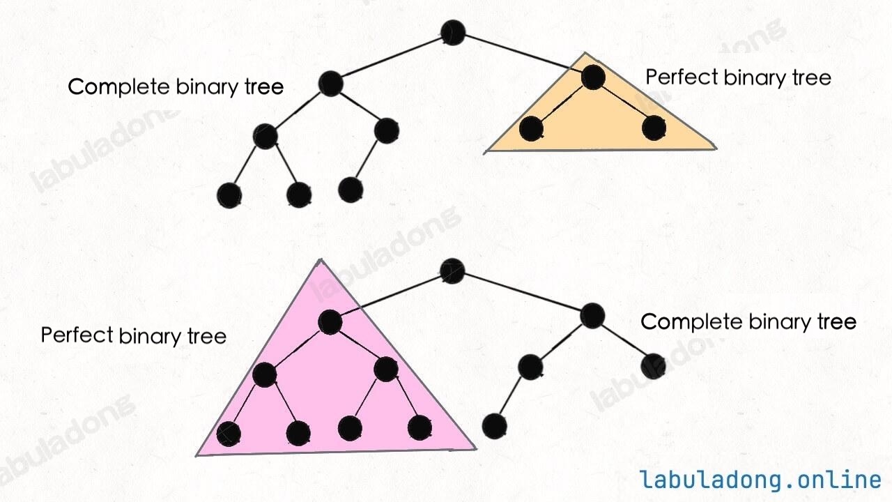
Complete Binary Tree

A complete binary tree is one where all levels are fully filled except possibly for the last level, which must be filled from left to right:

It's not hard to see that a full binary tree is a special kind of complete binary tree.

Characteristics of a complete binary tree: Due to its compact arrangement, there is a clear pattern in the indexing of parent and child nodes when numbered from left to right, top to bottom.

This characteristic is used when discussing the core principles of binary heap and core principles of segment tree: a complete binary tree can be stored using an array, without needing to actually construct linked nodes.

A less obvious property of a complete binary tree is: The left and right subtrees of a complete binary tree are also complete binary trees.

Or more accurately: At least one of the left or right subtrees of a complete binary tree is a full binary tree.

This property is used in algorithm problems, such as efficiently calculating the number of nodes in a complete binary tree, which will be mentioned here briefly.

Binary Search Tree

A Binary Search Tree (BST) is a common type of binary tree defined as follows:

For each node in the tree, the value of every node in its left subtree must be less than the value of that node, and the value of every node in its right subtree must be greater. You can simply remember this as "left smaller, right larger."

I emphasized "every node in the subtree" because beginners often make the mistake of focusing only on child nodes rather than all nodes in the entire subtree.

For example, the following is a BST:

All node values in the left subtree of node 7 are less than 7, and all node values in the right subtree are greater than 7. Similarly, all node values in the left subtree of node 4 are less than 4, and all node values in the right subtree are greater than 4.

Conversely, the following tree is not a BST:

If you only focus on each node's left and right children, you might not see the issue. However, you should consider the entire subtree; note that there's a node 8 in the left subtree of node 7, which is greater than 7, violating the BST definition.

BST is a highly useful data structure. Its "left smaller, right larger" property allows quick location of a specific node or all nodes within a range, which is the advantage of a BST.

For instance, in an ordinary binary tree with no specific order among nodes, finding a node with value x requires a full traversal starting from the root.

In a BST, you can compare the root node with x. If x is greater than the root node, you can immediately exclude the entire left subtree and start searching in the right subtree, quickly locating the node with value x.

There will be a dedicated chapter with detailed explanations and numerous exercises on BSTs later, but for now, these basic concepts will suffice.

Height-Balanced Binary Tree

A balanced binary tree is a special kind of binary tree where the height difference between the left and right subtrees of every node does not exceed 1.

Note that this applies to every node, not just the root.

For example, in the binary tree below, the root node 1 has a left subtree height of 2 and a right subtree height of 3; node 2 has a left subtree height of 1 and a right subtree height of 0; node 3 has a left subtree height of 2 and a right subtree height of 1. For every node, the height difference between the left and right subtrees does not exceed 1, so this is a balanced binary tree:

The following tree is not a balanced binary tree because node 2 has a left subtree height of 2 and a right subtree height of 0. The height difference is greater than 1, which does not meet the condition:

If there are $N$ nodes in a balanced binary tree, its height is $O(\log N)$ . This is a very important property. In later chapters, we will discuss several data structures based on binary trees. If the height of the tree can be kept at $O(\log N)$ , then operations such as insertion, deletion, search, and update will be very efficient.

On the other hand, if the tree is highly unbalanced, for example:

This tree is essentially a singly linked list, so the efficiency of insertion, deletion, search, and update operations in the tree will be greatly reduced.

Self-Balancing Binary Tree

We introduced balanced binary trees above, mentioning that their height is $O(\log N)$ and that operations on them are efficient.

Therefore, we can adjust the structure of the tree when inserting or deleting nodes, so that the tree always remains balanced. There are many kinds of self-balancing binary trees. The most classic example is the Red-Black Tree, which is a self-balancing binary search tree.

The key to keeping a tree balanced is the "rotation" operation. The visual panel below demonstrates the rotation operation in a Red-Black Tree. You can click on the left and right rotation code to see the effect of the rotations:

Algorithm Visualization

Implementation of Binary Trees

The most common binary tree is similar to a linked list, using a linked storage structure where each binary tree node has pointers to its left and right child nodes. This method is straightforward and intuitive.

On LeetCode, the binary trees you are given as input are generally constructed using this method. The TreeNode class for binary tree nodes typically looks like this:

java

class TreeNode {
    int val;
    TreeNode left;
    TreeNode right;
    TreeNode(int x) { this.val = x; }
}

// You can construct a binary tree like this:
TreeNode root = new TreeNode(1);
root.left = new TreeNode(2);
root.right = new TreeNode(3);
root.left.left = new TreeNode(4);
root.right.left = new TreeNode(5);
root.right.right = new TreeNode(6);

// The constructed binary tree looks like this:
//     1
//    / \
//   2   3
//  /   / \
// 4   5   6

cpp

class TreeNode {
public:
    int val;
    TreeNode* left;
    TreeNode* right;
    TreeNode(int x) : val(x), left(nullptr), right(nullptr) {}
};

// You can construct a binary tree like this:
TreeNode* root = new TreeNode(1);
root->left = new TreeNode(2);
root->right = new TreeNode(3);
root->left->left = new TreeNode(4);
root->right->left = new TreeNode(5);
root->right->right = new TreeNode(6);

// The constructed binary tree is like this:
//     1
//    / \
//   2   3
//  /   / \
// 4   5   6

python

class TreeNode:
    def __init__(self, x: int):
        self.val = x
        self.left = None
        self.right = None

# You can build a binary tree like this:
root = TreeNode(1)
root.left = TreeNode(2)
root.right = TreeNode(3)
root.left.left = TreeNode(4)
root.right.left = TreeNode(5)
root.right.right = TreeNode(6)

# The constructed binary tree looks like this:
#     1
#    / \
#   2   3
#  /   / \
# 4   5   6

type TreeNode struct {
    Val   int
    Left  *TreeNode
    Right *TreeNode
}

// You can construct a binary tree like this:
root := &TreeNode{Val: 1}
root.Left := &TreeNode{Val: 2}
root.Right := &TreeNode{Val: 3}
root.Left.Left := &TreeNode{Val: 4}
root.Right.Left := &TreeNode{Val: 5}
root.Right.Right := &TreeNode{Val: 6}

// The constructed binary tree looks like this:
//     1
//    / \
//   2   3
//  /   / \
// 4   5   6

javascript

var TreeNode = function(x) {
    this.val = x;
    this.left = null;
    this.right = null;
}

// you can construct a binary tree like this:
var root = new TreeNode(1);
root.left = new TreeNode(2);
root.right = new TreeNode(3);
root.left.left = new TreeNode(4);
root.right.left = new TreeNode(5);
root.right.right = new TreeNode(6);

// the constructed binary tree looks like this:
//     1
//    / \
//   2   3
//  /   / \
// 4   5   6

Since the above is a common implementation method, it implies there are other methods, right?

Yes, in Principles and Implementation of Binary Heap and Detailed Explanation of Union-Find Algorithm, we choose to use arrays to store binary trees based on specific needs.

When visualizing recursive functions in the Visualization Panel, a recursive tree is generated from the function stack, which can also be considered a way to implement binary trees.

Moreover, in typical algorithm problems, we may abstract the real-world problem into a binary tree structure, but we don't necessarily need to create a binary tree using TreeNode. Instead, we can represent binary/multi-way trees using structures similar to a hash table.

For example, consider the binary tree above:

I can use a hash table where the keys are parent node ids and the values are lists of child node ids (each node's id is unique). A key-value pair represents a multi-way tree node, and this multi-way tree can be represented as:

java

// 1 -> [2, 3]
// 2 -> [4]
// 3 -> [5, 6]

HashMap<Integer, List<Integer>> tree = new HashMap<>();
tree.put(1, Arrays.asList(2, 3));
tree.put(2, Collections.singletonList(4));
tree.put(3, Arrays.asList(5, 6));

cpp

// 1 -> {2, 3}
// 2 -> {4}
// 3 -> {5, 6}

unordered_map<int, vector<int>> tree;
tree[1] = {2, 3};
tree[2] = {4};
tree[3] = {5, 6};

python

# 1 -> [2, 3]
# 2 -> [4]
# 3 -> [5, 6]

tree = {
    1: [2, 3],
    2: [4],
    3: [5, 6]
}

// 1 -> [2, 3]
// 2 -> [4]
// 3 -> [5, 6]

tree := map[int][]int{
    1: {2, 3},
    2: {4},
    3: {5, 6},
}

javascript

// 1 -> [2, 3]
// 2 -> [4]
// 3 -> [5, 6]

let tree = new Map([
    [1, [2, 3]],
    [2, [4]],
    [3, [5, 6]]
]);

This way, you can simulate and manipulate binary tree/multi-way tree structures. When we discuss graph theory later, you will learn that it has a new name called Adjacency List.